Antenna Models
This topic provides technical information on some of the antenna models used by STK Communications and STK Radar. Use the following links to see information for a specific type:
- Parabolic
- Gaussian
- Square Horn
- Cosine Squared Pedestal Aperture
- Sinc
- Pencil Beam
- Dipole
- Helix
- Bessel Circular Aperture
- Bessel Envelope
- ITU Patterns
- GIMROC Files
Parabolic antenna
The parabolic antenna parameters are:
d = diameter of the parabolic dish
λ = wavelength
The gain of a parabolic antenna is modeled by the following equations:
This model is for a uniformly illuminated circular aperture dish. For further discussion of the parabolic model, see the section on technical notes.
See Maral, G., and M. Bousquet, Satellite Communications Systems: Systems, Techniques and Technology, 2nd ed., Chichester: Wiley (1993), sec. 2.1.3; Gagliardi, Robert M., Satellite Communications, 2nd ed., New York: Van Nostrand Reinhold (1991), sec. 3.2.
Gaussian antenna
The Gaussian antenna parameters are:
d = dish diameter
ρa = aperture efficiency
λ = wavelength
Θ3dB =3 dB beamwidth
The gain of the Gaussian antenna is modeled by the equation:
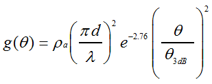
The value for 3 dB beamwidth is an approximation. See below for further discussion of this and other aspects of the Gaussian model.
Gagliardi, Robert M., Satellite Communications, 2nd ed., New York: Van Nostrand Reinhold (1991), p. 104.
Square horn antenna
The square horn antenna parameters are:
d = length of the side of the square horn
λ = wavelength
The square horn antenna's gain is modeled by the following equations:
Gagliardi, Robert M., Satellite Communications, 2nd ed., New York: Van Nostrand Reinhold (1991), p. 102.
Cosine squared pedestal aperture
The radiation distribution is:
where z ranges from to and Pʋ is the pedestal value.
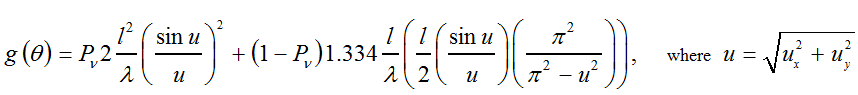
Sinc
For the sinc power N model, the gain pattern is as follows:
where N is the exponent.
The equations for 3 dB beamwidth (degrees) for cosine and cosine squared antennas are:
Cosine
Cosine squared
The pedestal add-on is given by:
For the 3 dB beamwidth of a sinc power N model, use
where
The maximum gain for the cosine and cosine squared models is calculated with the following equations (unless you enter a value):
Cosine
Cosine squared
For the pedestal versions, add
For the sinc power N model, maximum gain defaults to zero if you do not enter a value.
See Balanis, Constantine, Antenna Theory: Analysis and Design, New York: Wiley (1982), pp. 690-694; and Raemer, Harold R., Radar Systems Principles, Boca Raton: CRC Press (1997), pp. 349-356.
Pencil beam antenna
For the pencil beam antenna, the main lobe gain, beamwidth, and side lobe gain relationships are given by:
where BW = beamwidth
When modeling off-normal array effects,
where GENDFIRE = minimum gain as function of angle off normal.
The maximum off-normal angle is given by:
For Θ < ΘMax,
For Θ ≥ ΘMax,
Hansen, R.C., Phased Array Antennas, New York: Wiley (1998), sec. 2.4.4.
Dipole antenna
The dipole antenna parameters are:
L = full length of the dipole
Θ = angle off the boresight
The gain pattern is obtained from the normalized directivity D of the radiation intensity function F of the dipole antenna, as given by the following equations:
Numerical integration with 180 steps provides a good approximation to the integral.
Balanis, Constantine, Antenna Theory: Analysis and Design, New York: Wiley (1982), secs. 4.5.3 and 4.5.4.
Helix antenna (Comm)
The helical antenna parameters are:
d = diameter of helix
C = circumference of helix =πd
S = turn spacing
α = pitch angle = tan-1 (S/C)
N = number of helix turns
L = length of helix = NS
Θ = elevation angle off the boresight
STK models only uniform diameter helices and the axial mode of operation. Directivity is given by:
The normalized far field antenna pattern is:
where
These relations yield good approximations, provided that 12° < α < 15°, 3/4 < C/λ < 4/3, and N ≈ 3-100.
Balanis, Constantine, Antenna Theory: Analysis and Design, New York: Wiley (1982), pp. 386-92.
Bessel circular aperture antennas
The following parameters apply to Bessel circular apertures:
diameter of circular aperture, D = 2α
α = radius at edge of aperture
ρ = radius at any point on aperture
p = πρ/α
μ = 2α sin θ/λ = D/λ sin θ
A = 10(EdgePad/20)
B = 1 - A
The circular aperture voltage antenna pattern is defined by the following equation:
where
g(p) = Aperture Distribution Function= A + B (1-p2)z
where Z = one of the following values:
0 (Uniform Illumination)
1 (Parabolic Illumination)
2 (Parabolic Squared Illumination)
A value of 0 dB for EdgePad will also force the illumination to be uniform across the aperture.
J0(ρμ)= Bessel function of the first kind of zero order
The normalized far field voltage Bessel pattern is given by:
The above equations are provided courtesy of Bill Brasile at MRJ Technology Solutions.
Bessel envelope pattern
The asymptotic form of the Bessel function is given by:
Substituting the envelope function into the normalized Bessel power pattern, and letting
yields the following expression for the envelope of the normalized power Bessel pattern:
Complex Bessel Function Envelope
Amplitude Adjustment
The asymptotic nature of the envelope curve gives very high values near the boresight. The following procedure determines the tangent of the envelope curve to the Bessel function pattern. Bessel function pattern gain values are used below this tangent point.
The following is an illustration of the Bessel envelope pattern:

The above equations and illustration are provided courtesy of Bill Brasile at MRJ Technology Solutions.
ITU antenna patterns
Notes on the side lobe mask level parameter
AGI provides the side lobe mask level parameter to enable you to set the side lobe mask level independently of the peak gain of the main lobe, when using the ITU S465-5, S580-5 and S731 antenna masks. These patterns have the form G(Θ) = A - B log(Θ) for Θ > Θmin and G(Θ) = MaxGain for Θ < Θmin. The side lobe mask level value you supply is set equal to A in the preceding equation. You can see an example of this, using the S465-5 pattern, in the following figure.
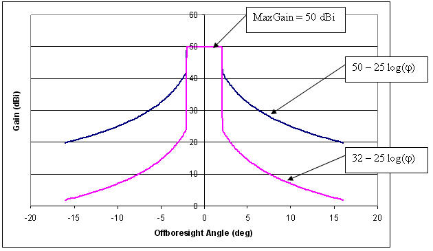
As you can see from the figure, both antenna patterns have a peak main lobe gain of 50 dBi. The difference is that one of the masks has a side lobe mask described by 50 - 25 log(Θ) and the other by 32 - 25 log(Θ). This was achieved by setting the side lobe mask level parameter to 50 and 32 dBi respectively.
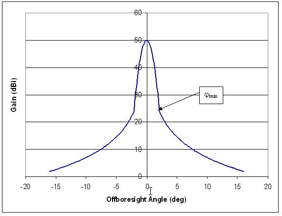
Notes on the ITU radio regulations main lobe model
The main lobe (Θ ≥ 0 and Θ < Θmin) is not defined for many of the ITU antenna pattern recommendations. STK models this region, by default, as a constant or flat gain at the main lobe peak gain value you supply. Alternatively, you can choose to model this region using the ITU Radio Regulations Appendix 8 main lobe model [G(Θ) = Gmax - 0.0025 * ((D/λ>*Θ)2].
GIMROC contour files
The following comments expand on the limitations that you may encounter when importing ITU GIMROC antenna contour files into STK.
Background
ITU GIMROC satellite antenna files are sample data points of antenna gain contours projected onto the surface of the Earth. The data points are recorded in terms of latitude and longitude. The resolution of the data points is limited, and in some cases only a few (1-4) contours are provided.
There is very little additional information available with GIMROC files regarding antenna dish type and size. The transmitter frequency used for generating the gain contours is generally not known. Some contours are generated by multiple beam antennas and are due to the aggregate gain of several beams. Additional problems may arise due to the off-axis orientation of spot beams.
The actual maximum gain of the antenna is not known; the contours represent relative gain only. Antenna boresight is always the 0 dB reference.
Importing GIMROC files into STK
STK generates antenna contours using analytical gain models. Where these models are unavailable, STK reads the gain data matrix from an external file. The gain data may be a set of measurements on an actual antenna. STK uses the gain data to generate the 3D models of antenna gain in STK 3D Graphics and to project 2D contours onto the surface of the Earth or onto a hypothetical surface at a given altitude.
In the case of ITU GIMROC data, actual antenna information is missing. STK reads in the contour data and uses a 3D interpolation process to approximate an antenna beam gain matrix. This process yields only an estimate of the best possible fit for the antenna gain matrix. The accuracy of the curve/surface fit is highly dependent on the number of contours and the number of points per contour. Larger data sets will help to improve the estimated results but will still provide only an approximation of the actual antenna gain.
STK uses this estimated gain matrix, just as it uses those generated by analytical gain models, to generate the projections of contours. Unlike the analytical model, this matrix remains constant at all times. A change of transmitter frequency or antenna characteristics has no impact on the gain matrix and the generated contours.
On the other hand, the beam generated on the basis of GIMROC data behaves similarly to analytical model beams in several respects. For example, you can orient it like a normal beam, and you can study the effects of satellite dynamics, wave polarization, etc.
The gain contours generated by GIMROC antenna files in STK are not a copy of the contours read in from the GIMROC (*.gxt) files. STK contours are generated by an antenna gain matrix computed by STK. This matrix is an approximation based on contour sample data read from the GIMROC files.
Differences between the original data points and the contours produced by STK are due to the following factors:
- Only a limited data set is available in the ITU GIMROC database.
- The process of interpolation is an estimation of a surface from limited 2D data to a 3D high-resolution antenna gain matrix.
- Original satellite location may be different than the location of the satellite that is reading in the data.
- Satellite antenna orientation may be different than the orientation of the satellite that is reading in the data.
The process of curve fitting a data set is an approximate best fit. The objective of the process is to minimize the discrepancy between the actual data and the estimated surface points. STK achieves this where the original data points exist. Outside that region, STK estimates the surface points by extrapolation of the best-fit curve/surface. Since no data points exist in this region, there is no criterion for minimizing the error; hence, the contours generated by STK are likely to show a wider variation.
You should weigh this marginal loss of accuracy against the advantages of using the analytic capabilities offered by STK.
Further notes on parabolic and Gaussian antenna models
If you are familiar with STK sensor patterns, you may be interested in knowing how those patterns relate to the antenna models provided by STK Communications and STK Radar. For example, the half-power sensor models a parabolic dish, using a cone angle calculated on the basis of a nonuniform illumination law:
where Θ3dB = 3 dB beamwidth, λ = wavelength, D = diameter of dish, c = speed of light, and f = frequency (Hz)
AGI chose 70 degrees on the basis of the illumination law. You can achieve a uniform illumination by using 58.5 degrees instead.
The simpler relation described previously for the Gaussian beam is adequate out to about the 6 dB beamwidth. Since this model factors the efficiency into the 3 dB beamwidth, it enables you to model different illumination types, where an efficiency of 1.0 is equivalent to a uniformly illuminated antenna. The relationship between the efficiency of the Gaussian antenna and the 3 dB antenna contour is evident from the fact that the efficiency appears in the denominator in the equation that gives us the approximation of Θ3dB:
where ρa = antenna efficiency factor.
This relationship does not apply to the parabolic model, which is for a uniformly illuminated dish.
Thus, an important difference between the 3 dB beamwidth for the Gaussian and parabolic models is the way in which they model illumination. The Gaussian approximation gives you some control over the amount of illumination, using the efficiency factor in the user interface, while the parabolic model forces it to be uniform.
The difference between the half-power sensor and STK Communications and STK Radar antenna models can also be attributed to the differences between the illumination laws used. In contrast to the Comm/Radar parabolic model, the half-power sensor is not uniformly illuminated, due to the choice of 70 degrees instead of 58.5 degrees. However, you can make the illumination of the Gaussian model uniform or nonuniform by varying the efficiency factor. With the efficiency set at 0.67, the Gaussian model will produce a 3 dB pattern equivalent to that produced by the half-power sensor model. You can see this by setting the two above equations for Θ3dB as equal and solving for the efficiency factor.
Maral, G., and M. Bousquet, Satellite Communications Systems: Systems, Techniques and Technology, 2nd ed., Chichester: Wiley (1993), sec. 2.1.3; Gagliardi, Robert M., Satellite Communications, 2nd ed., New York: Van Nostrand Reinhold (1991), pp. 101-04.