STK Premium (Air), STK Premium (Space), or STK Enterprise
You can obtain the necessary licenses for this training by contacting AGI Support at support@agi.com or 1-800-924-7244.
This lesson requires STK 12.5 or newer to complete because it includes new features introduced in STK 12.5.
The EOIR installation package is included with the STK Premium installation package. However, you must install EOIR on your computer separately from the STK application. See the EOIR capability help for more information.
Pictures, graphs, and data snippets are used as examples only. The results of the tutorial may vary depending on the user settings and data enabled (online operations, terrain server, dynamic Earth data, etc.). It is acceptable to have different results.
Capabilities covered
This lesson covers the following STK Capabilities:
- STK Pro
- Electro-Optical Infrared Sensor Performance (EOIR)
Problem statement
Engineers and operators need to understand how their on-board cameras will behave within the mission context. They want to simulate what a sensor will see if it looks at a different target under different conditions, which is important. If they own the sensor, field tests are expensive and complicated, results are uncertain, and there are no do-overs. If they don't own the sensor, they may want a better understanding of what kind of results it can achieve or perhaps what kind of threat it might present. Many simulation tools are proprietary, classified, or compartmented. STK's EOIR capability is an available commercial-off-the-shelf (COTS) solution.
Solution
You will use STK's Electro-Optical Infrared (EOIR) capability to create a realistic model of a ground imaging sensor from reference images. First you will reconstruct a specific scene with known location and timing and insert an artificial object into the scene. This will result in a sensor image with the target object overlaid on the reference background image. You will use the image to perform in-scene calibration of the sensor and target models. Once you have an acceptably accurate model, you will then explore the potential performance of the sensor in varying conditions. The conditions will include the impact of various atmospheric models and parameters, as well as illumination conditions, including low light.
External files
This lesson will walk through how to use MATLAB to convert a file. Any utility that converts an image file into a CSV file will work for this study.
However, the converted files are available for download via one of the following methods:
- Download the three files from the STK Data Federate, AGI Support - Virtual Training - AGI Training Scenarios - Lesson Specific Files - EOIR Sensor Calibration Ground Imaging directory
- Click the links below and download each file:
What you will learn
Upon completion of this tutorial, you will be able to:
- Create system models such as satellite orbits, EO/IR system specs, and sample target objects.
- Load custom image texture maps into your STK scenario.
- Conduct in-scene model calibrations with regard to the resolution and sensitivity.
Video guidance
Watch the following video. Then follow the steps below, which incorporate the systems and missions you work on (sample inputs provided).
Creating a new scenario
Create a new scenario with a run time of one day.
- Launch STK (
 ).
). - Click .
- Enter the following in the STK: New Scenario Wizard:
- Click when you finish.
- Click Save (
 ) when the scenario loads. A folder with the same name as your scenario is created for you.
 - Verify the scenario name and location shown in the Save As window.
- Click .
| Option | Value |
|---|---|
| Name | Ground_Imaging_EOIR |
| Start |
30 Jul 2017 00:00:00.000 UTCG |
| Stop | + 1 day |
Save often!
Verify that EOIR is installed
Ensure that EOIR is installed on your computer. If you do not have the EOIR Toolbar, check the status of your license and whether you have EOIR installed.
- Look for the EOIR toolbar (
 ) in your STK GUI.
 - Extend the View menu if you do not see the EOIR toolbar ( ).
- Select Toolbars.
- Select EOIR.
Disabling Terrain Server
You will not be using the streaming terrain for this analysis. Disable it in the scenario properties.
- Open Ground_Imaging_EOIR's (
 ) properties (
 ).
). - Select the Basic – Terrain page.
- Clear the Use terrain server for analysis check box.
- Click to accept the changes and close the Properties Browser.
Inserting a satellite
You will use SkySat-C3 (SSCN 41774), a satellite launched by Planet, in your mission to image the ground. Insert this satellite into your scenario from the Standard Object Database.
- Select Satellite (
 ) in the Insert STK Objects tool.
 - Select the From Standard Object Database (
 ) method.
 - Click .
- Enter 41774 into the Name or ID field.
- Click .
- Select the Skysat-C3 from the AGI’s Standard Object Data Service data source.
- Click .
- Click when done.
Modeling the Boston Logan airport
Insert Boston into the scenario. You will move the place object to the tarmac near the Boston Logan airport terminals. This will be the "target" for the camera on board Skysat-C3.
Inserting a Place object
Insert Boston into the scenario.
- Select Place (
 ) in the Insert STK Objects tool.
 - Select the From City Database () method.
- Click .
- Enter Boston into the Name field.
- Click .
- Select Boston, Massachusetts. You’ll move this point after it’s inserted.
- Click .
- Click when done.
Relocating the place
Change the location of the place object to the tarmac near the Boston Logan airport terminals.
- Open Boston's (
 ) properties ().
 - Select the Basic - Position page.
- Enter 42.364 deg for the Latitude.
- Enter -71.0244 deg for the Longitude.
- Click .
Setting the scenario animation time
Modify the scenario time to match the “acquired” time of the image. From an external source, you know that during the below specified period, the Sky Sat was overhead and was able to capture an image of the ground.
- Open Ground_Imaging_EOIR's () properties ().
- Select the Basic - Time page.
- Clear the Use Analysis Start Time check box in the Animation section.
- Enter 30 Jul 2017 15:32:11.507 UTCG in the Start Time field.
- Click .
- Click Reset (
 ) in the Animation toolbar.
You can also update the animation time directly in the Animation toolbar.
Computing Access
Now that the time is set, compute access from SkySat to Boston.
- Right-click SKYSAT-C3_41774 () in the Object Browser.
- Select Access... (
 ).
). - Ensure the SkySat satellite is selected in the Access for field.
- Select Boston () in the Associated Objects list.
- Click Compute (
 ).
).
Finding the view angle
Generate an AER report to find the elevation angle at the time above.
- Click in the Reports section of the Access () window.
- Scroll to the 30 Jul 2017 15:32:11.507 UTCG time step.
- Make note of the Elevation Angle. It is about -77 deg. This is a good angle to view the ground site.
Modeling an EO/IR sensor
Next you will insert a sensor to model EO/IR capabilities. You will keep the default settings for the sensor, but you will reduce the size of the field of view. You don't have to have every specification to start, you can begin with a general model and refine the settings throughout the analysis.
Inserting a Sensor object
Insert a sensor to model EO/IR capabilities.
- Select Sensor (
 ) in the Insert STK Objects tool.
 - Select the Define Properties () method.
- Click .
- Select SKYSAT-C3_41774 in the Select Object list.
- Click .
- Right-click Sensor1 ( ) in the Object Browser.
- Select Rename.
- Rename Sensor1 ( ) Default_EOIR_1deg.
Updating the sensor type
Update the sensor's properties to model an EOIR Sensor Type with a 1 deg field of view.
- Select the Basic - Definition page in Default_EOIR_1deg's () properties.
- Set the Sensor Type to EOIR.
- Ensure the Spatial tab is selected on the Basic - Definition page.
- Set the following options:
Option Valure Input Field-of-View and Number of Pixels Field of View - Horizontal Half Angle 1 deg Field of View - Vertical Half Angle 1 deg - Click .
Pointing to Boston
Update the sensor's properties to point to Boston.
- Go to the Basic - Pointing page.
- Set the Pointing Type to Along Vector.
- Click next to the Alignment vector field.
- Select SKYSAT-C3_41774/Default_EOIR_1deg () on the left of the Select Alignment Vector window.
- Expand (
 ) To Vectors on the right.
 - Select Boston (
 ).
). - Click .
- Click to close the sensor's Properties Browser.
You didn't simply target the ground object. That's because you want to orient the view so that north is at the top of the image. This is a preference and aligns with the general approach of placing north at the top of a map.
Generating a sensor scene
Create an EOIR sensor scene for this sensor at the animation time you set earlier in the lesson (30 Jul 2017 15:32:11.507 UTCG).
Generating an image of the sensor output
Generate an image that represents the sensor output.
- Select the Default_EOIR_1deg ( ) in the Object Browser.
- Click the EOIR Sensor Scene (
 ) button in the EOIR toolbar to generate an image that represents the sensor output. Give STK a moment to generate the scene.
 - Right-click the sensor scene.
- Select Details...
- Select Scene Detail – Fine.
- Click .
- Examine the view. You should now see the default Earth background texture. This 1 km texture map that comes with EOIR is adequate for very broad area applications.
Changing the color map
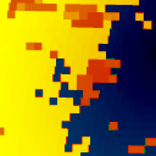
Change the color map.
- Select Color Map – BGRY in the EOIR Scene Visual Details window.
- Click . Areas that were varying shades of gray are now red, orange, green, brown, and blue.
- Click the different colors in the scene. Note the Material type in the EOIR Scene Visual Details window change depending on which part of the scene you have selected. As you click, you should see various kinds of materials listed in the field including Urban, WaterBody, GrassLands, and more.
- Select Color Map – Gray Scale in the EOIR Scene Visual Details window.
- Click .
Next, examine the reflectance maps.
Creating the reflectance map
Texture maps, like the reflectance map you will use in this lesson, can come from your own sources or you can create them from within STK. Below, you will walk through a work flow for creating your own maps. The example file will be generated from Bing data, which only has red, green, and blue data. You will use the data you have available and extend it to whichever wavebands you use in this study. Please note, the example file has already been converted and is available on the SDF. The link to the file is in this lesson's External Files section.
To create your own image, follow the below procedure for your area of interest. STK's Bing imagery and the snap frame capability is a good option.
Creating the Stored View
Create a Stored View of Boston.
- Right-click Boston () in the Object Browser.
- Select Zoom To.
- Zoom out slightly in the 3D Graphics window, so your view looks something like this:

It is ok if your airport looks different than the picture above. STK automatically updates ground imagery with the latest Bing imagery available. If you want the same imagery as above, you can load in the image file provided on the SDF above (airport.jp2) to the 3D Graphics display. You can also use your own imagery file. Please review the Working with Imagery Help page.
- Click Stored Views (
 ) in the 3D Graphics toolbar.
 - Click .
- Change the View Name of view to Boston.
- Click .
- You need to note the corner latitude and longitude points.Use your cursor on the 3D Graphics window or define an area target so you can capture this information. The example reflectance file has the following corner points:
Point Latitude (deg) Longitude (deg) NW Corner 42.3654 -71.0271 NE Corner 42.3654 -71.0232 SW Corner 42.3631 -71.0271 SE Corner 42.3631 -71.0232
Snapping the frame
Take a snapshot of your 3D Graphics window view.
- Clear up the 3D Graphics window by disabling any visualized object and removing any annotations or overlays.
- Click Snap Properties (
 ) on the 3D Graphics toolbar.
 - Select Snap to File for the Capture option.
- Review the settings and make any changes to the resolution of the output file.
- Click Snap Frame (
 )
) - Set the File Name to Airport.bmp.
- Save the file in your scenario directory.
Converting the image into a CSV file
Convert the file you just created into a CSV file. Your image has three channels (red, green, and blue). You can copy and modify the following MATLAB code for use to normalize across each channel. The MATLAB script below was used to create Airport.csv. You can create your own CSV file or use the one downloaded earlier.
- Open MATLAB.
- Copy the following script into MATLAB, replacing C:\ with the location of your BMP file
a=imread('C:\Airport.bmp');b=mean(a,3);
imagesc(b)
b=b/max(b(:));
csvwrite('C:\Airport.csv',b); - Press Enter on your keyboard.
- Go to your directory where you saved Airport.csv to confirm that is has been created.
Importing the reflectance map
After downloading the example files, or creating your own, load the file into your scenario for your camera to view.
Opening EOIR Configuration window
Open the EOIR Configuration window.
- Click the EOIR Configuration (
 ) button on the EOIR toolbar.
 - Click .
- Select the Texture Maps page.
- Click New Texture Map (
 ).
). - Set the following:
Option Value Name Reflectance Type Reflectance
Loading the texture map file
Load in the texture map file.
- Change the Value drop-down menu selection to File.
- Click the ellipsis (
 ) beside the File: field.
 - Browse to and select the Airport.csv file.
- Click .
- Set the corner points using the values you noted above or from the table below.
Point Latitude (deg) Longitude (deg) NW Corner 42.3654 -71.0271 NE Corner 42.3654 -71.0232 SW Corner 42.3631 -71.0271 SE Corner 42.3631 -71.0232 - Click . Give STK a moment to load the file.
- Click to close the EOIR Configuration window.
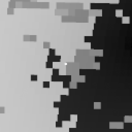
Revisiting the sensor scene
Examine the changes in the EOIR Sensor Scene window. If closed, reopen the EOIR Sensor scene. Otherwise, if it was open, then the scene will automatically update. Examine the changes.
- Select the Default_EOIR_1deg ( ) in the Object Browser.
- Click the EOIR Sensor Scene ( ) icon in the EOIR toolbar to generate an image that represents the sensor output. Give STK a moment to generate the scene.
- Examine the scene. You will see the custom imagery overlaid on the default Earth background:
You can improve EO/IR sensor realism with published specs and some engineering understanding. The following references provide some helpful information about the SkySat imager:
- https://earth.esa.int/eogateway/news/improved-resolution-for-skysat-data-and-extension-of-planet-data-availability
- https://earth.esa.int/eogateway/missions/skysat
- https://www.int-arch-photogramm-remote-sens-spatial-inf-sci.net/XL-1/95/2014/isprsarchives-XL-1-95-2014.pdf
Summarizing some relevant details
Here are some relevant details:
- The EO/IR sensor has an effective nadir resolution (also called Ground Sample Distance, or GSD) at 450km of 50 cm after super resolution processing. See GSD formula documentation.
- The optics has a 3.6 m focal length and 35 cm aperture.
- The effective detector pitch value you get from solving the GSD equation using the values above is 4.0 μm. However, one of the sources gives a value of 6.5 μm. This gives you a range of values to begin with.
Creating a new sensor on the SkySat satellite
You will begin to refine your EO/IR System specs. The system specs can come from open source or published documentation, as you will use here. Over the course of the lesson, you will look at the aperture and focal length, modify the spectral bands, modify the optical and radiometric inputs, and examine the detector pitch.
Inserting a Sensor object
Insert a sensor to model EO/IR capabilities.
- Select Sensor ( ) in the Insert STK Objects tool.
- Select the Define Properties () method.
- Click .
- Select SKYSAT-C3_41774 in the Select Object list.
- Click .
- Rename Sensor1 ( ) SkySat_EOIR.
Updating the sensor type
Update the sensor's properties to model an EOIR Sensor Type.
- Select the Basic - Definition page in SkySat_EOIR's () properties.
- Set the Sensor Type to EOIR.
- Ensure the Spatial tab is selected on the Basic - Definition page.
- Rename Band1 to PAN.
- Click .
Setting the spatial properties
Set the number of pixels to 128 x 128 and detector pitch to 6.5 μm. Even though the SkySat sensor has a much higher pixel count, considering only a subset of its image area will speed up the processing. You can also do this because you will ensure STK points the sensor directly at the desired target and will not need to search a large scene to find it.
- Ensure the Spatial tab is selected on the Basic - Definition page.
- Set the Input to Number of Pixels and Detector Pitch.
- Set the following:
Option Value Number of Pixels - Horizontal 128 Number of Pixels - Vertical 128 Related Detector Parameters - Hoirz Pixel Pitch 6.5 um Related Detector Parameters - Vertical Pixel Pitch 6.5 um
Setting the spectral properties
Set the shortest and longest wavelengths that the sensor responds to.
- Select the Spectral tab.
- Set the following:
Option Value Low 0.45 um High 0.90 um
Setting the optical properties
Set the optical parameters.
- Select the Optical tab.
- Set the following:
Option Value Input Focal Length and Entrance Pupil Diameter Effective Focal Length 350 cm Entrance Pupil Diameter 35 cm - Click .
Pointing to Boston
Update the sensor's properties to point to Boston.
- Go to the Basic - Pointing page.
- Set the Pointing Type to Along Vector.
- Click next to the Alignment vector field.
- Select SKYSAT-C3_41774/SkySat_EOIR () on the left of the Select Alignment Vector window.
- Expand () To Vectors on the right.
- Select Boston ().
- Click .
- Click to close the sensor's Properties Browser.
Modeling an aircraft object near the airport to image
Now, model a target object, in this case an aircraft parked at the airport. As you can see from the Airport.bmp image, you have two aircraft parked on the tarmac. Load your own aircraft into the scenario, so you can compare it to what the sensor sees in the ground imagery.
Inserting an Aircraft object
Create an aircraft parked at a terminal beside an aircraft image, for comparison.
- Select Aircraft (
 ) in the Insert STK Objects tool.
 - Select the Define Properties () method.
- Click .
- Rename Aircraft1 () 737.
Setting the aircraft's location
Park the aircraft at a terminal for one day.
- Click on the Basic - Route page.
- Set the following:
Option Value Route Calculation Method Specify Time Altitude Reference - Reference WGS84 Latitude 42.36384740 deg Longitude -71.02423046 deg Altitude 3 m You can also create the first point using 2D or 3D object editing.
- Click .
- Set 31 Jul 2017 00:01:00.000 UTCG as the Time for the second point so it is one day later.
- Go to the 3D Graphics - Vector page.
- Select the Show check box for Sun Vector.
- Click .
- Examine the 3D Graphics window to verify the results. In the 3D Graphics window, especially at this angle, you can distinguish your inserted aircraft from the aircraft on the ground. For now, focus the sensor in this direction and examine what it would see in the scene.

Defining the EO/IR shape of the aircraft
EOIR supports custom 3D mesh files, either user-supplied or from the STK install . It’s important to use realistic dimensions for the 3D model you choose, as EOIR will scale the model to match the Max Dimension you enter.
- Select the Basic - EOIR Shape page in the Aircraft's Properties ().
- Set the following:
Option Value Shape CustomMesh Max Dimension 37 m Mesh File C:\Program Files\AGI\STK 12\EOIR_Databases\PropertyFiles\CustomMeshes\Air\Boeing-737.obj Material Gray Body Reflectance 25% - Click .
Adding the aircraft object to the EOIR configuration
Now that the aircraft is defined, set up the EO/IR sensor so it sees it.
- Click the EOIR Configuration () button on the EOIR toolbar.
- Select Aircraft/737 () in the list of Available STK Objects.
- Click Move (
 ) to move Aircraft/737 () to the list of Selected Targets.
 - Click .
Getting the 737 inside the EO/IR sensor frame
The SkySat sensor is already targeted to Boston, so use 3D Object Editing to reposition its coordinates between the 737 aircraft and an adjacent aircraft in the background image. Note, when moving Boston, you can alternatively set the position values on Boston's Basic - Position page. Latitude 42.364 deg, Longitude -71.0244 deg works well.
- Bring the 3D Graphics window to the front.
- Select Place/Boston in the 3D Object Editor 3D Editing Object drop-down list.
- Click Object Edit Start/Accept (
 ) to start the editing process.
 - Press the Shift key on your keyboard.
- Left-click near the aircraft to move the Place object to that location.
- Click Object Edit Start/Accept (
 ) to start the editing process.
 - Notice in the 3D Graphics window that your aircraft and the aircraft from the image are both in the EO/IR sensor's field-of-view.

Creating a stored view
A stored view makes it easy to get back to the specific time at which you want to render your image.
- Set your scenario time to 30 Jul 2017 15:32:11.507 UTCG (if not already set).
- Bring the 3D Graphics window to the front.
- Click Stored Views () in the 3D Graphics toolbar.
- Click .
- Change the View Name to Tarmac.
- Click .
Generating a sensor scene
Create an EOIR sensor scene. You are now ready to see how well you did!
Generating an image of the sensor output
Generate an image that represents the sensor output.
- Select the SkySat_EOIR ( ) in the Object Browser.
- Click EOIR Sensor Scene ( ) in the EOIR toolbar to generate an image that represents the radiometric input to the sensor. Give STK a moment to generate the scene.
- Right-click the sensor scene.
- Select Details...
- Select Scene Detail – Fine.
- Click .
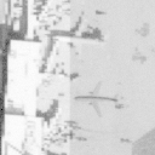
- Examine the scene. The 737 aircraft object should now appear within the scene:
- Compare the two aircraft in the scene. Although the EOIR target aircraft (737) looks very similar to the aircraft in the image, there are a few differences worth noting.

Exploring the shadows:
EOIR does not render shadows cast from custom 3D mesh objects onto the ground or onto themselves, such as the vertical stabilizer onto the horizontal stabilizer. However, you can see that the proper side of the fuselage is shaded due to the sun’s position and is consistent with other objects in the background image.
- Look at the 737's fuselage in the scene.
- Notice the proper side of the fuselage is shaded due to the sun’s position. This is consistent with the other objects' shading in the background image.
Exploring the scene contrast
The shaded regions of the EOIR aircraft fuselage show a darker black than almost any other part of the scene. This is especially noticeable between comparable locations on the aircraft fuselage in the background image. There are a couple of potential reasons for this:
- EOIR does not compute reflections from the sky, which will result in less ambient light and thus starker shadows.
- The white balance of the background image could be a bit off. One approach to work around this is to convert the image background to a percentile map. Essentially, it will cut out the top 5% brightest and top 5% darkest pixels and rescale the reflectance values accordingly. This is a crude approximation of scaling the image to the dark pixel and light pixel reflectance values, or using the Emperical Line Method (ELM) to calibrate all pixel values. You can do this in MATLAB by recreating the CSV file. You will add a few commands to the end of the code you used above. The additional commands are in bold below. The script in the section below was used to create Airport_v2.csv.
Create the new Airport_v2.csv file. Then load it into your scenario.
Scaling the image
Cut out the top 5% brightest and top 5% darkest pixels and rescale the reflectance values accordingly. The MATLAB script below was used to create Airport_v2.csv. You can create your own CSV file or use the one downloaded earlier.
- Open MATLAB.
- Copy the below script into MATLAB replacing C:\ with the location of your BMP file
a=imread('C:\Airport.bmp');b=mean(a,3);
imagesc(b)
b=b/max(b(:));
b=b-0.1;
b(b<0)=0;
csvwrite('C:\Airport_v2.csv',b); - Press Enter on your keyboard.
Loading the texture map file
Load in the new texture map file.
- Return to your STK scenario.
- Click the EOIR Configuration () button on the EOIR toolbar.
- Click .
- Select the Texture Maps page.
- Click the ellipsis () beside the File: field.
- Browse to and select the Airport_v2.csv file.
- Click .
- Click . Give STK a moment to load the file.
- Click to close the EOIR Configuration window. Your EOIR scene will look like this. The darkness from the EOIR target aircraft’s shaded fuselage is now much closer to that of the background image.
Changing 737's target reflectance
Besides the shadows, the 737 aircraft itself still appears a little darker than the adjacent aircraft. This could easily be due to the actual reflectance of the real aircraft in the background image, paint color, surface treatments, etc. If your goal is to create an aircraft that matches the imaged aircraft even more closely, you could change the 737’s EOIR Shape Reflectance value to 22%. For more advanced applications, you may want to supply a Spectral Reflectance File. For more information, see the EOIR General Vehicle Shape Properties help page.
- Right-click 787 (
 ) in the Object Browser.
 - Select Properties ().
- Select the Basic - EOIR Shape page.
- Set Reflectance to 22%
- Click .
Investigating 737's target edge sharpness
The 737 aircraft seems to be slightly sharper or more “in focus” than the rest of the scene, especially at the wings. Part of the reason may be that your EOIR sensor model is using a few idealized parameters. One of these parameters is jitter along the line of sight. It is currently set to 0 milliradians, or a perfectly stable platform. A more appropriate value for a real platform might be 0.1 to 1.0 times the Instantaneous FOV of a single pixel. For 128 x 128 pixels and 6.5 μm pixel pitch, the IFOV is 0.0019 mrad. Set the Line of Sight Jitter to 0.001 mrad, or about 0.5 times the IFOV.
- Right-click SkySat_EOIR (
 ) in the Object Browser.
 - Select Properties ().
- Go to the Basic - Definition page.
- Set the Line of Sight Jitter to 0.001 mrad.
- Click .
- Examine your sensor scene. The scene now looks very blurred.

Now that you’ve been able to insert a false object into a collected image that is fairly consistent with an actual target, you can declare victory for your model calibration!
Comparing the scene
Compare the sensor scene with the 3D Graphics window.
- Compare the EOIR sensor scene above and your simulated 737 aircraft object to the 3D Graphics display. Optionally, you can open the saved Airport.bmp file outside of STK, which would better preserve the original pixilation.
- Compare the apparent resolution, or Ground Sample Distance (GSD), between the two images.
- Compare the detail in the scene. Is there enough detail in the scene to discern the various 737 variants or a 737 from an Airbus A320?
- Examine the scene to determine if the scenario produces a sufficiently accurate model of this sensor's performance. Does this give you confidence in evaluating the sensor performance in other scenes and against other targets?

Verifying the sensor resolution
Earlier in the exercise, you found a potential range of values to use for detector pitch, and thus, GSD. You initially picked the largest value, 6.5 μm, for detector pitch. Now is a good time to revisit that assumption. You can also reference the earlier SkySat sensor parameters and find the detector pitch required to achieve 0.8 m/pixel for the sensor. STK Pro includes the ability to compute GSD geometrically for accesses involving a sensor object when you specify the Sensor Properties – Basic – Resolution values of Focal Length and Detector Pitch.
Updating sensor properties
Update the sensor's focal length and detector pitch.
- Right-click SkySat_EOIR () in the Object Browser.
- Select Properties ().
- Select the Basic - Resolution page.
- Set the following:
Option Value Focal Length 3.5 m Detector Pitch 6.5 um - Click .
Computing Access
Compute access from SkySat_EOIR to Boston.
- Right-click SkySat_EOIR () in the Object Browser.
- Select Access... ().
- Select Boston () in the Associated Objects list.
- Click Compute ().
Creating a new report
Create a new report to display constraint data.
- Click in the Access window to open the Report & Graph Manager.
- Click Create new report style (
 ) in the Styles toolbar.
 - Name the report GSD.
- Press Enter on your keyboard.
- Expand (
 ) Constraint Data (
 ) in the Data Provider list.
 - Move () the following elements from the Constraint Data Access data providers:
Data Provider Time ToElevationAngle
The elevation angle will change depending on if you compute access from the ground to the satellite versus from the satellite to the ground. When computing FROM SkySat’s sensor TO Boston, use the ToElevationAngle to get elevation of SkySat above Earth’s horizon.
FromRange FromGroundSampleDistance - Click .
Analyzing the Ground Sampling Distance (GSD)
Generate a Dynamic Display to analyze the GSD.
- Confirm or set the scenario animation time to 30 Jul 2017 15:32:11.507 .
- Right-click the GSD (
 ) report in the My Styles list.
 - Select Generate Dynamic Display.
- STK computes a GSD of 0.97 m for this shot.
- Change Detector Pitch to 5.3 um in SkySat_EOIR's () Basic - Resolution properties page.
- Click .
- Return to the GSD Dynamic Display. STK now computes a GSD of 0.79 m for this shot. If you refer to the SkySat Sensor parameters linked earlier in the lesson, you find yourself in close range to the values reported by Planet.
- Set the following in SkySat_EOIR's () Basic - Definition properties page:
Option Value Related Detector Parameters - Hoirz Pixel Pitch 5.3 um Related Detector Parameters - Vertical Pixel Pitch 5.3 um - Click .
This now represents a more accurate effective detector pitch for this image.
Verifying the GSD computation
In addition to inspecting the pixels in the sensor scene, EOIR also computes a relevant value in its “EOIR Sensor to Target Metrics” data providers. The target is selected by the EOIR configuration toolbar button.
Verifying the target is selected
- Click the EOIR Configuration () button on the EOIR toolbar.
- Confirm that the 737 () aircraft is listed as an Available STK Objects.
- Click .
Creating a new report
Create a new report to display GSD data.
- Right-click SkySat_EOIR () in the Object Browser.
- Select Report & Graph Manager.
- Click Create new report style () in the Styles toolbar.
- Name the report EOIR metrics.
- Press Enter on your keyboard.
- Expand () EOIR Sensor to Target Metrics () in the Data Provider list.
- Move () the following elements from the EOIR Sensor to Target Metrics data providers:
Data Provider Time Range to Target Geometric instantaneous field of view footprint - Click .
Analyzing the Ground Sampling Distance (GSD)
Generate a Dynamic Display to analyze GSD.
- Right-click the EOIR metrics () report in the My Styles list.
- Select Generate Dynamic Display.
EOIR sensor-to-target metrics compute more slowly than many other data providers. Be careful not to create a standard report using the default object time period and time step, as this would require significant computational time. The Dynamic Display computes these values only for the current time step.
- STK computes a Geometric Instantaneous field of view footprint of 0.615 at the time of the stored view. Assuming a square pixel, the square root of 0.615 is 0.784 m, in the range of the GSD values reported by Planet.
Examining the impact of atmospheric model
You will next run some stress tests on the system. All of your work up to this point has not used any atmospheric models at all. You can verify this by looking in the EOIR configuration's (![]() ) Atmosphere Definition page.
) Atmosphere Definition page.
EOIR includes a Simple Atmosphere and a MODTRAN Atmosphere model. Both models take the same input parameters: Aerosol models, Visibility, and Humidity. Begin by seeing what impact atmospheric modeling will have on the specific scene you have been recreating. To do this, you should use the most appropriate Aerosol, Visibility, and Humidity models and values for the time and location being imaged. Historical humidity and visibility information for Boston can be found online, for example here, https://www.wunderground.com/history/daily/us/ma/boston/KBOS/date/2017-7-30. The Visibility was 10 miles (16 km) and Humidity was 55%. Boston Logan is on Boston Harbor, so the Urban Aerosol Model is probably most appropriate.
You will generate two more scenes: one using the Simple Atmosphere model and one using MODTRAN Atmosphere model. Then, you will compare these two scenes with the one previously created that did not use an atmospheric model.
Setting the Simple Atmosphere model
Set the atmospheric properties for the generated sensor scene to use the Simple Atmosphere model.
- Select SkySat_EOIR () sensor in the Object Browser.
- Click the EOIR Configuration () button on the EOIR toolbar.
- Click .
- Set the following on the Atmosphere page:
Option Value Atmosphere Modes Simple Atmosphere Aerosol Models Urban Visibility 16.0 km Humidity 55% - Click to close the EOIR Atmosphere, Clouds, and Texture maps window.
- Click to close the EOIR Configuration window.
- Look at your regenerated sensor scene. If you closed your sensor scene, click EOIR Sensor Scene ( ) in the EOIR toolbar to generate an image.
Setting the MODTRAN Atmosphere model
Set the atmospheric properties for the generated sensor scene to use the MODTRAN Atmosphere model.
- Select SkySat_EOIR () sensor in the Object Browser.
- Click the EOIR Configuration () button on the EOIR toolbar.
- Click .
- Set the following on the Atmosphere page:
Option Value Atmosphere Modes MODTRAN Atmosphere Aerosol Models Urban Visibility 16.0 km Humidity 55% - Click to close the EOIR Atmosphere, Clouds, and Texture maps window.
- Click to close the EOIR Configuration window.
- Look at your regenerated sensor scene. Note the increase in processing time when using MODTRAN.
You’ll notice there is only a minor difference in the image quality for these images. This is because the image was taken when SkySat C3 was about 77 deg above the horizon, and relatively little atmosphere was in the way.
Examining other atmospheric settings on your own
On your own, examine the image quality with the other atmospheric settings. Here are some examples to try:
- Try Simple Atmosphere test cases:
Option Test Cases A Test Cases B Test Cases C Test Cases D Atmosphere Modes Simple Atmosphere Simple Atmosphere Simple Atmosphere Simple Atmosphere Aerosol Models Urban Urban Rural Rural Visibility 5 km, 10 km, 15 km, 30 km 10 km 5 km, 10 km, 15 km, 30 km 10 km Humidity 55% 15%, 50%, 85% 55% 15%, 50%, 85% - Try MODTRAN Atmosphere test cases:
Option Test Cases A Test Cases B Test Cases C Test Cases D Atmosphere Modes MODTRAN Atmosphere MODTRAN Atmosphere MODTRAN Atmosphere MODTRAN Atmosphere Aerosol Models Urban Urban Rural Rural Visibility 5 km, 10 km, 15 km, 30 km 10 km 5 km, 10 km, 15 km, 30 km 10 km Humidity 55% 15%, 50%, 85% 55% 15%, 50%, 85% - Determine if atmospheric conditions change the answers to the above questions about detection or identification.
- Examine the image quality with a different elevation angle. You took your images at an elevation angle of about 77 deg. Consider what your scene would look like at a lower elevation angle.
Determining lunar phase
Thus far, you have imaged the aircraft during the daytime. Next you will find some nighttime imaging opportunities under a full Moon.
You will make some modifications to the scenario, including extending the scenario time, adding constraints, modifying the aircraft, and creating stored views.
Updating the scenario time period
- Right-click Ground_Imaging_EOIR () in the Object Browser.
- Select Properties ().
- Set Analysis Period - Stop time to +30 days on the Basic - Time tab. This will let you consider the entire month for desired conditions.
- Click .
Analytically calculate the lunar phase
Use STK's Analysis Workbench capability to create a new angle. The new angle will calculate the angle between the Moon-Earth vector and the Moon-Sun vector.
- Click the Analysis Workbench (
 ) icon in the STK Tools toolbar.
 - Select the Vector Geometry.
- Select Primary Central Bodies in the Filter by drop-down list.
- Select Moon (
 ) in the Objects list.
 - Click Create New Angle (
 ).
). - Set the following:
Option Value Type Between Vectors Name Phase From Vector Moon Earth To Vector Moon Sun - Click to close the Add Geometry Component window.
- Click to close the Analysis Workbench.
Constraining Access
Use Access Constraints to find a good SkySat imaging opportunity with a nearly full Moon above the horizon.
Setting Sun constraints
Set Sun constraints so Access can only occur with a nearly full Moon above the horizon.
- Right-click Boston () in the Object Browser.
- Select Properties ().
- Select the Constraints - Sun page.
- Set the following:
Option Value Sun Elevation Angle - Max -5 deg (the Sun must be 5 deg or more below the horizon) Lunar Elevation Angle - Min 1 deg (the Moon must be 1 deg or more above the horizon)
Setting a phase angle constraint
Set a 15 deg max phase angle constraint.
- Select the Constraints - Vector page.
- Click .
- Select Primary Central Bodies in the Filter by drop-down list.
- Select Moon () in the Objects list.
- Select Phase () in the Components for: Moon list on the right.
- Click .
- Clear Moon Phase Angle - Min.
- Set the Moon Phase Angle - Max to 15 deg. This constrains the highest allowable phase angle to 15 deg. A phase angle of 0 deg would correspond to a perfectly “full” Moon.
- Click .
Computing access elevation angles from Boston
Examine the max elevation angle when Boston and SkySat (![]() ) have Access.
) have Access.
- Right-click Boston () in the Object Browser.
- Select Access... ().
- Select SKYSAT-C3_41774 () in the Associated Objects list.
- Select Use Scenario Time Period.
- Click in the Reports section of the Access () window.
- Examine the Max Elevation statistics to find the highest Max Elevation near 88.5 deg on 8 Aug 2017 02:38:09.578 UTCG. This result may differ depending on the placement of the Boston place object.
- Right-click the time in the report.
- Select Time.
- Select Set Animation Time.
- Using the 3D window, verify that SkySat C3 is directly overhead, the Sun is below the horizon, and Moon is above the horizon and appears full from Boston.
Creating a stored view
Create a stored view at this animation time called Full Moon Access. Having a stored view makes it easy to get back to the specific time at which you want to render your image.
- Bring the 3D Graphics window to the front.
- If you are not zoomed in on Boston, Zoom to Boson.
- Click Stored Views () in the 3D Graphics toolbar.
- Click .
- Change the View Name to Full Moon Access.
- Click .
Modifying target aircraft properties
Make the aircraft static for the full range of lighting conditions.
- Right-click 737() in the Object Browser.
- Select Properties ().
- Go to the Basic - Route page.
- Ensure the Route Calculation Method is set to Specify Time.
- Confirm that the first waypoint has a start time at 30 Jul 2017 00:00:00 UTCG.
- Set the time of the second waypoint to 30 Aug 2017 03:00:00 UTCG. Recall that you extended the scenario stop time to 30 days, so you are making a similar update here.
Generating a sensor scene
Generate a sensor scene with the new constraints.
- Extend the Stored Views () drop-down menu.
- Select Full Moon Access.
- Select SkySat_EOIR () sensor in the Object Browser.
- Click the EOIR Configuration () button on the EOIR toolbar.
- Click .
- Select Atmosphere Off.
- Click to close the EOIR Atmosphere, Clouds, and Texture maps window.
- Click to close the EOIR Configuration window.
- Click EOIR Sensor Scene ( ) in the EOIR toolbar to generate an image. Typically, with a full Moon there is enough light for the human eye to very easily make out distinct shapes and shadows and identify common objects. See how your EOIR sensor does.

It doesn’t look like much, does it? The settings used for this image are the default values:
- Noise Equivalent Radiance: 1e-15 @ 100 msec
- Saturation Equivalent Irradiance: 3e-12 @ 100 msec
- Dynamic Range: 3000
- Integration Time: 100 msec
The sensor thus is either not sensitive enough or simply not getting enough photons. You will need to make some adjustments to the sensitivity and integration time to get a usable image.
Modifying sensitivity
Adjust the sensitivity (noise floor, or lowest detectable signal) and dynamic range (ratio of lowest to highest detectable signal) to compensate. To do this, you’ll need to determine the highest and lowest signal values in our scene, essentially the radiance values in the brightest and darkest pixels. Since there isn’t much to see in your sensor scene, tell EOIR to render the Radiometric Input to the sensor — all the information EOIR computes about all the photons — right before it hits your detector array.
Modeling radiometric input
Change the EOIR sensor's Processing Level to Radiometric Input.
- Right-click SkySat_EOIR () in the Object Browser.
- Select Properties ().
- Go to the Basic - Definition page.
- Change Processing Level from Sensor Output to Radiometric Input.
- Click .
Examining the sensor scene
Examine the sensor scene.
- Bring the sensor scene to the front. It is automatically updated.
- Right-click anywhere in the scene.
- Select Details…
- Click the darkest part of the scene, somewhere in the shaded side of the target aircraft fuselage.
- Take note of the Inband Radiance value.
- Repeat the previous step, but for the brightest part of the scene, somewhere in the moonlit side of the fuselage.

Updating Radiometric properties
Update the EOIR sensor's Radiometric properties based on what you just observed.
- Return to SkySat_EOIR's () Basic - Definition Properties () page.
- Select the Radiometric tab.
- Select Radiance for the Units for Saturation and Sensitivity. This will match the units of the values we just measured.
- Set 5.7e-12 for the Sensitivity - EquivalentValue for the 100 msec Integration Time. This is the dark pixel value. This is the lowest detectable signal above the noise floor for a 100 msec integration time.
- Set 5.8e-9 for the Dynamic Range - EquivalentValue for the 100 msec Integration Time. This is the bright pixel value. This is the maximum detectable signal before the array is saturated.
- Change Processing Level back to Sensor Output.
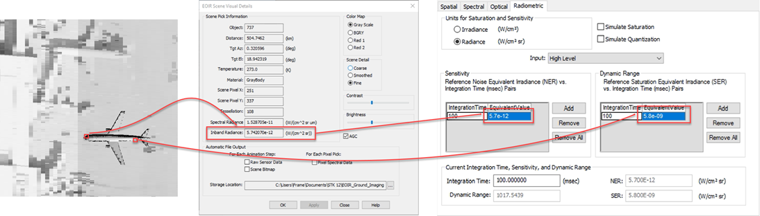
- Click .
Examining the sensor scene
Examine the sensor scene.
- Bring the sensor scene to the front. It is automatically updated to something like this:
- Examine the image. The image is no longer just static, and you can make out some straight lines and brighter and darker regions. With a little difficulty you may be able to recognize the building and some items on the tarmac. But it’s still not a very useable image.

Getting more photons
If you’ve ever tried to do any astrophotography and image a dim object like a nebula or galaxy, you’ll know there are really only two ways to get more photons: you can increase the aperture or increase the exposure time. Your aperture is fixed at 35 cm based on specifications, but you can change the exposure time.
- Return to SkySat_EOIR's () Basic - Definition Properties () page.
- Select the Radiometric tab.
- Set the Integration Time to 500 msec.
- Click .
- The sensor scene should update to look something like this:

This is much better! The aircraft fuselage is clearly visible, and the wings are even somewhat discernible.
Adding more realism
So far so good, but see what happens when you add a bit more realism to the simulation. You'll do this by simulating quantization. This is especially important for low-light situations because you may be getting only a very few photons from the scene. This is the analog to digital converter. Before you may have been simulating half a photon, which would let you see artificially exaggerated resolution within the scene. With quantization on, you either get an electron out of your detector array, or you don’t, due to the quantum mechanical nature of photons and electrons.
Simulating quantization
Update the EOIR sensor to simulate quantization.
- Return to SkySat_EOIR's () Basic - Definition Properties () page.
- Select the Radiometric tab.
- Select Simulate Quantization. Turning on Quantization simulates the analog-to-digital conversion at the detector.
- Click .
Setting the atmosphere model
Set the atmosphere model to represent very good “seeing” conditions. Recall that for the daytime scene, adding an atmospheric model at high elevations had a minimal impact.
- Select SkySat_EOIR () sensor in the Object Browser.
- Click the EOIR Configuration () button on the EOIR toolbar.
- Click .
- Set the following on the Atmosphere page:
Option Value Atmosphere Modes Simple Atmosphere Aerosol Models Urban Visibility 30 km Humidity 15% - Click to close the EOIR Atmosphere, Clouds, and Texture maps window.
- Click to close the EOIR Configuration window.
- Look at your regenerated sensor scene. It should look something like this:

The image quality is noticeably degraded. This is understandable given our low-light and atmospheric settings.
As you can see, through an iterative process you're able to add realism to your scene. You can adjust the scene here further to balance the gray scale through the Radiometric settings. On your own, use the work flow you've learned to tweak the image.
Save your work
- When finished, close any reports, graphs, and tools that are still open.
- Save (
 ) your work.
Conclusion
Using STK's EOIR modeling capabilities, you have been able to create a realistic model of a ground imaging sensor. You began with default settings and iterated to a detailed setup. Using a sample ground image, you performed in-scene calibrations of the sensor and target model. Once set up, you were able to stress test the sensor's capability, such as including poor collection conditions versus nominal conditions and varying lighting conditions.
On your own
On your own, explore the effects of atmospheric conditions on the sensor scene. If you have your own ground image, calculate the GSD by measuring a known object (such as street width) in both pixels and distance, as defined in STK. Use your results to calibrate the EOIR sensor. You examined a nighttime scene with a full moon; now reexamine the scenario but with a new Moon overhead.