Part 10:
STK Premium (Air), STK Premium (Space), or STK Enterprise
You can obtain the necessary licenses for this training by contacting AGI Support at support@agi.com or 1-800-924-7244.
Additional installation - Analyzer. You can obtain the necessary install by visiting http://support.agi.com/downloads or calling AGI support.
The results of the tutorial may vary depending on the user settings and data enabled (online operations, terrain server, dynamic Earth data, etc.). It is acceptable to have different results.
Capabilities Covered
This lesson covers the following STK Capabilities:
- STK Pro
- Coverage
- STK Analyzer
Problem
Engineers and operators require a quick way to determine how various orbital parameters such as semi-major axis, eccentricity, inclination, argument of perigee, right ascension of the ascending node or true anomaly will effect the ability of a sensor or camera to view the surface of the Earth. In this lesson, you want to quickly run multiple trade studies to determine how inclination, eccentricity or a combination of both will effect the percentage of coverage over the entire Earth during a 24 hour period.
Solution
Use STK Pro and STK's Coverage and Analyzer capabilities to run Parametric and Carpet Plot analyses. The studies will determine the best combination of inclination and eccentricity that provides the highest percentage of global coverage.
What you will learn
Upon completion of this tutorial, you will understand:
- Analyzer
- Analyzer parametric studies
- Analyzer carpet plots
Video Guidance
Watch the following video. Then follow the steps below, which incorporate the systems and missions you work on (sample inputs provided).
Create a New Scenario
Create a new scenario.
- Launch STK (
 ).
). - In the Welcome to STK window, click Create a Scenario (
 ).
). - Enter the following in the New Scenario Wizard:
- When you finish, click OK.
- When the scenario loads, click Save (
 ). A folder with the same name as your scenario is created for you in the location specified above.
 - Verify the scenario name and location and click Save.
| Option | Value |
|---|---|
| Name: | STK_Analyzer |
| Location: | Default |
| Start: | 1 Jul 2020 16:00:00.000 UTCG |
| Stop: | 2 Jul 2020 16:00:00.000 UTCG |
Save (![]() ) often!
) often!
View Both the 2D and 3D Graphics Windows
You can view coverage in both the 2D and 3D Graphics windows. Placing them side by side makes this simple to do.
- Close the Time Line at the bottom of STK.
- Click Window in the STK menu bar.
- Select Tile Vertically.
Turn Off Terrain Server
Analytical and visual terrain is not required in this analysis.
- Open STK_Analyzer's () properties (
 ).
). - Select the Basic - Terrain page.
- Clear the Use terrain server for analysis option.
- Click OK to accept the changes, and close the Properties Browser.
Design a Satellite Orbit
Insert a Satellite (![]() ) object, and place it in a retrograde orbit. Use the Orbit Wizard Orbit Designer which allows you to create a custom orbit.
) object, and place it in a retrograde orbit. Use the Orbit Wizard Orbit Designer which allows you to create a custom orbit.
- Using the Insert STK Objects tool, insert a Satellite (
 ) object using the Orbit Wizard (
 )method.
 - Set the following:
- Click .
| Option | Value |
|---|---|
| Type: | Orbit Designer |
| Satellite Name: | MySat |
| Semimajor Axis: | 10600 km |
| Eccentricity: | 0.363 |
| Inclination: | 116 deg |
| Argument of Perigee: | 270 deg |
| RAAN: | 104 deg |
| True Anomaly: | 90 deg |
Sensor Object
Use a Sensor (![]() ) object that provides a simple conic, 20 degree, field-of-view. The field of view will simulate a camera's field-of-view.
) object that provides a simple conic, 20 degree, field-of-view. The field of view will simulate a camera's field-of-view.
- Using the Insert STK Objects tool, insert a Sensor (
 ) object using the Define Properties () method.
 - When the Select Object window opens, select MySat ().
- Click OK.
- On the Basic - Definition page, change the Simple Conic - Cone Half Angle: value to 10 deg.
- Click OK to accept the changes, and close the Properties Browser.
- Rename the Sensor () object Camera_View.
Coverage Definition Object
The Coverage Definition object defines a coverage area for analysis. In this instance, you require global coverage.
- Using the Insert STK Objects tool, insert a Coverage Definition (
 ) object using the Insert Default method.
 - Rename the Coverage Definition () object Global_Grid.
- Open Global_Grid's () properties ().
Coverage Grid
Global Coverage grid type creates a grid that covers the entire globe.
- On the Basic - Grid page, change Grid Area of Interest - Type: to Global.
- Click Apply to accept the changes, and keep the Properties Browser open.
Coverage Assets
Assets properties allow you to specify the STK objects used to provide coverage.
- Select the Basic - Assets page.
- In the Assets list, select Camera_View ().
- Click Assign.
- Click OK to accept the changes, and close the Properties Browser.
Figures of Merit
A Figure of Merit (![]() ) object allows you to specify the method by which the quality of coverage is measured. The default Coverage type for a Figure Of Merit (
) object allows you to specify the method by which the quality of coverage is measured. The default Coverage type for a Figure Of Merit (![]() ) object is simple coverage.
) object is simple coverage.
- Using the Insert STK Objects tool, insert a Figure Of Merit (
 ) object using the Insert Default method.
 - When the Select Object window opens, select Global_Grid ().
- Click OK.
- Rename the Figure Of Merit () object Simple_Cov.
Compute Accesses Tool
The ultimate goal of Coverage is to analyze accesses to an area using assigned assets.
- Right-click Global_Grid () in the Object Browser.
- Select CoverageDefinition.
- Select Compute Accesses.
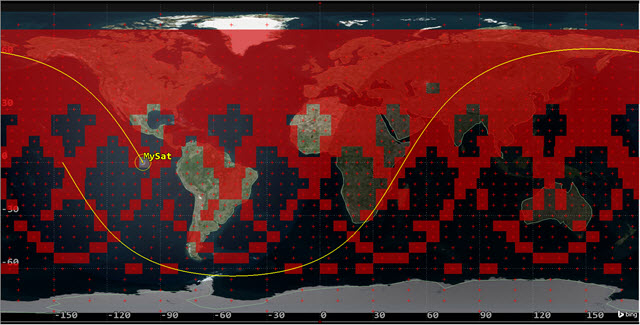
2D Graphics Window Global Coverage
Percent Satisfied
Percent Satisfied is the percentage of coverage grid area which is satisfied. It's computed by summing the areas associated with all satisfied grid points, dividing by the total grid area and multiplying by 100. In this scenario, you're interested in the Percent Coverage static value of Simple Coverage, meaning the percent of the coverage grid area covered by at least one asset at some point during the coverage interval.
- Right-click on Simple_Cov () in the Object Browser.
- Select Report & Graph Manager (
 ).
). - When the Report & Graph Manager opens, select the Percent Satisfied report in the Installed Styles list.
- Click Generate.
- Note the % Satisfied value at the bottom of the report (e.g. ~49 percent). The value you see is the scenario benchmark.
- When finished, close the report and the Report & Graph Manager.
Analyzer
Analyzer provides a set of analysis tools that:
- Enable you to understand the design space of your systems.
- Enable you to perform analyses in STK easily, without involving programming or scripting.
- Introduce trade study and post-processing capabilities.
- Can be used with all STK scenarios, including those with STK Astrogator satellites.
Determine the Impact of Satellite Inclination on Percent Satisfied
The first study you will perform varies inclination and its effect on global coverage. You need to select input and output variables from the main Analyzer window to pass to the Parametric Study tool.
- Click View on the STK menu bar.
- Select Toolbars.
- Select Analyzer.
- Click the Analyzer (
 ) button on the Analyzer Tool Bar.
Another way of opening Analyzer is to click Analysis on the STK menu bar, select Analyzer, and then click the Analyzer button. One more way opening Analyzer is to go to the Object Browser, right-click on the object (or any object), select the object's Plugins, and click Analyzer.
Analyzer Layout
Use the Analyzer Main Form to configure input and output variables available for further analysis. You will first select an object in the STK Variables tree on the left. When an object is selected, all possible input variable candidates are listed under the STK Property Variables - General tab and the Active Constraints tab. All output variable candidates are listed under the Data Provider Variable - Data Providers tab and Object Coverage tab.
Input Inclination
Start by selecting Inclination as the Input variable.
- Select MySat () in the STK Variables tree.
- Expand (
 ) Propagator (TwoBody) in the STK Property Variables - General tab.
 - Double-click on Inclination to move it to the Analyzer Variables field as an Input.
Output Percent Satisfied
The same data providers that are in the Report & Graph Manager are available in the Data Provider Variables list. Select Percent Satisfied as the Output variable.
- In the STK Variables tree, expand () Global_Grid ().
- Select Simple_Cov ().
- Expand () Static Satisfaction in the Data Provider Variables - Data Providers tab.
- Double-click on Percent Satisfied to move it to the Analyzer Variables field as an Output.
Parametric Study Tool
The Parametric Study Tool runs a model through a sweep of values for some input variable. The resulting data can be plotted to view trends.
Let's set up a Parametric Study with Inclination as the Design Variable and Percent Satisfied as the Response.
- Click Parametric Study... (
 ) on the Analyzer toolbar to open the Parametric Study Tool.
 - Drag and drop the Design Variable, Inclination, from the Component Tree on the left to the Parametric Study Tool on the right.
- Set the following:
- Notice the number of samples is automatically calculated as nine based on the values we set.
- Drag and drop the Percent Satisfied data provider element into the Responses field.
- Click Run...
- Notice nine runs are performed since the number of samples is set to nine.
| Option | Value |
|---|---|
| starting value: | 112 |
| ending value: | 120 |
| step size: | 1 |
Design Variable units are not specified in Analyzer. Analyzer assumes the default units set in STK.
Running the data explorer
The Data Explorer is a Trade Study tool used to display data collected from STK. While data is being collected in the Table, the Data Explorer window displays a progress meter, a halt button, and the data. Once the Parametric study is complete, the Table page and 2D Scatter Plot display the collected data.
- When the Parametric study is finished, close the 2D Scatter Plot.
- Select the Table Page - Trade Study 1 - Data Explorer window to bring it to the front.
- Notice nine runs were performed at 1 deg increments from 112 deg to 120 deg inclination.
- Notice the second row shows the global coverage percentage for each change in inclination.
- Note that an inclination of 120 deg provides the highest percentage of global coverage.
- On the Table Page tool bar, click Add View.
- Select 2D Line plot.
- Click Axes.
- Select the Ticks tab.
- Change the Max # value to 20.
- Click anywhere on the plot to close the Axes menu.
- Looking at the 2D Line Plot, you see that 120 deg inclination (basing the analysis on one degree increments) gives you the best choice for global coverage during the 24 hour period.
- Close the 2D Line Plot and the Table Page.
- Select No when the Save window appears.
- Close the Parametric Study () window.
- Return to the Analyzer () window.
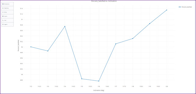
2D Line Plot Inclination
Input Eccentricity
Eccentricity could have an impact on the sensor's footprint. However, you have to take into consideration the possibility of the satellite impacting the Earth's surface when changing the eccentricity.
- Select MySat () in the STK Variables tree.
- In the STK Property Variables - General tab, expand () Propagator (TwoBody).
- Double-click on Eccentricity to move it to the Analyzer Variables field as an Input.
- Click the Parametric Study Tool () button on the Analyzer toolbar.
Eccentricity Parametric Study
Let's set up a Parametric Study with Eccentricity as the Design Variable and Percent Satisfied as the Response.
- Drag and drop the Design Variable, Eccentricity, from the Component Tree on the left to the Parametric Study Tool on the right.
- Set the following:
- Notice the step size is automatically calculated based on the values we set.
- Drag and drop the Percent Satisfied data provider element into the Responses field.
- Click Run...
| Option | Value |
|---|---|
| starting value: | .362 |
| ending value: | .364 |
| number of samples: | 10 |
Running the data explorer
- When the Parametric study is finished, close the 2D Scatter Plot.
- Select the Table Page - Trade Study 2 - Data Explorer window to bring it to the front.
- On the Table Page tool bar, click Add View.
- Select 2D Line plot.
- Click Axes.
- Select the Ticks tab.
- Change the Max # value to 40.
- Click anywhere on the plot to close the Axes menu.
- Place your cursor over one of the points. A small window will appear with analytical information concerning the point.
- Close the 2D Line Plot and the Table Page.
- Select No when the Save window appears.
- Close the Parametric Study () window.
- Return to the Analyzer () window.
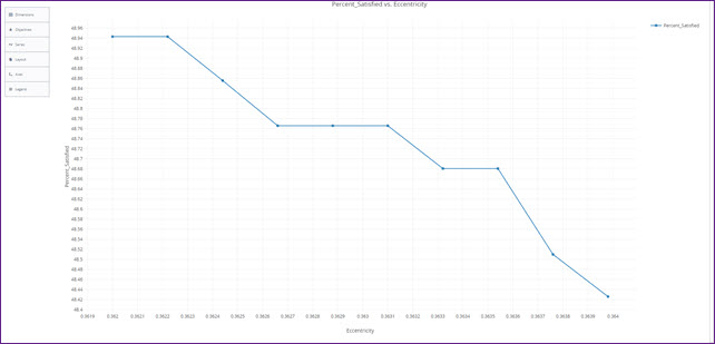
2D Line Plot Eccentricity
The small change in Eccentricity didn't have too much impact on global coverage. 0.362000 through 0.362220 provided a steady value of 48.9433 percent satisfied. After that, there is a steady drop in percentage.
Carpet Plot Tool
A Carpet Plot is a means of displaying data dependent on two variables in a format that makes interpretation easier than normal multiple curve plots. A Carpet Plot can be thought of as a multi-dimensional Parametric Study.
Let's set up a Carpet Plot with Inclination and Eccentricity as the Design Variables and Percent Satisfied as the Response. Setting the design variables is similar to using the Parametric Study Tool except you now have two variables instead of one.
- To access the Carpet Plot Tool (
 ), click Carpet Plot... on the Analyzer toolbar.
 - Drag and drop Inclination from the Component Tree on the left to the first Design Variable field on the right.
- Drag and drop Eccentricity from the Component Tree on the left to the second Design Variable field on the right.
- Set the following Inclination Design Variable:
- Set the following Eccentricity Design Variable:
- Drag and drop the Percent Satisfied data provider element into the Responses field.
- Click Run.
| Option | Value |
|---|---|
| From | 119 |
| To | 121 |
| Step Size | 1 |
| Option | Value |
|---|---|
| From | .361 |
| To | .365 |
| Step Size | 0.001 |
The Best Combination
Using the Carpet Plot Tool, look for the best combination of Inclination and Eccentricity. First, you will make the Carpet Plot easier to read, then look at the data.
- Click Axes.
- Select the Lines tab.
- Change the Grid Lines value to 10.
- Click anywhere on the plot to close the Axes menu.
- When finished, close the Carpet Plot and the Table Page.
- Select No when the Save window appears.
- Close the Carpet Plot Tool () window.
- Close Analyzer ().
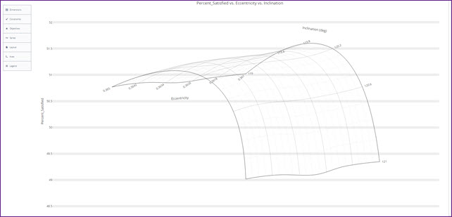
Percent Satisfied vs. Eccentricity vs. Inclination Carpet Plot
The original benchmark of global coverage was approximately 49 percent. In this study, an Inclination of 120 degrees and an Eccentricity of 0.361 provided the best percentage of global coverage of approximately 51.6 percent.
Summary
You began the scenario by placing a Satellite (![]() ) object in a retrograde orbit. You attached a Sensor (
) object in a retrograde orbit. You attached a Sensor (![]() ) object to the Satellite (
) object to the Satellite (![]() ) with a 20 degree field of view and orientated to point straight down below the Satellite (
) with a 20 degree field of view and orientated to point straight down below the Satellite (![]() ) to the Earth's surface. Using a Coverage Definition (
) to the Earth's surface. Using a Coverage Definition (![]() ) object, you created a global grid and assigned the Sensor (
) object, you created a global grid and assigned the Sensor (![]() ) object as the asset. Using a Figure Of Merit (
) object as the asset. Using a Figure Of Merit (![]() ) object and Simple Coverage, you determined that approximately 49 percent of the Earth's surface was accessed by the Sensor (
) object and Simple Coverage, you determined that approximately 49 percent of the Earth's surface was accessed by the Sensor (![]() ) object during a 24 hour analysis period. The Satellite's (
) object during a 24 hour analysis period. The Satellite's (![]() ) original Inclination was 116 degrees and its Eccentricity was 0.363. Using Analyzer, you ran two Parametric studies changing Inclination and Eccentricity and studied their effects on global coverage. You ended the analysis by running a Carpet Plot study which determined the best combination of Inclination and Eccentricity that provided the highest percentage of global coverage. Your final value for Inclination was 120 degrees and Eccentricity was 0.361. This combination raised global coverage percentage from the benchmark of approximately 49 percent to 51.6 percent.
) original Inclination was 116 degrees and its Eccentricity was 0.363. Using Analyzer, you ran two Parametric studies changing Inclination and Eccentricity and studied their effects on global coverage. You ended the analysis by running a Carpet Plot study which determined the best combination of Inclination and Eccentricity that provided the highest percentage of global coverage. Your final value for Inclination was 120 degrees and Eccentricity was 0.361. This combination raised global coverage percentage from the benchmark of approximately 49 percent to 51.6 percent.
On Your Own
You could rerun all the Parametric studies using new values with the existing input variables. You could add new inputs such as Semi Major Axis, and study how that affects coverage. A different approach might be to add an input that changes the cone half angle of the Sensor (![]() ) object. There are a lot of combinations you could try. Explore and have fun!
) object. There are a lot of combinations you could try. Explore and have fun!