STK Professional, Communications, Radar, Aviator, and Terrain Integrated Rough Earth Model (TIREM).
The results of the tutorial may vary depending on the user settings and data enabled (online operations, terrain server, dynamic Earth data, etc.). It is acceptable to have different results.
Problem Statement
You are conducting an exercise testing a surveillance radar system against a small single engine aircraftwhich is flying in rugged, mountainous terrain. An experimental aerostat containing a radar jamming package is tethered in a remote mountainous area 10,000 feet above ground level (AGL). Furthermore, you are testing whether or not the radar jammer on-board the aerostat can jam the surveillance radar.
Solution
Use Aviator to create a flight path using the STK Basic General Aviationmodel. Build a monostatic surveillance radar and create a custom graph to determine if you can track the aircraft. Build a simulated aerostat with an attached radar jam system. Using a custom graph, determine if the aerostat can jam the surveillance radar.
Create a New Scenario
Create a new scenario using the default analysis time period.
- Launch STK (
 ).
). - Create a scenario (
 ).
). - Name the scenario “Radar_Jamming.”
- Change Start: to 1 Jul 2016 16:00:00.000 UTCG.
- Change Stop: to 1 Jul 2016 18:00:00.000 UTCG.
SAVE OFTEN!
Add Terrain
- Open Radar_Jamming’s () properties (
 ).
). - Browse to the Basic – Terrain page.
- Turn off Use terrain server for analysis.
- Click OK.
- Bring the 3D Graphics window to the front.
- Launch the Globe Manager.
- Use the Add Terrain/Imagery option in the Globe Manager to load your terrain file (*.pdtt) to the globe in the 3D Graphics window.
- Browse to <STK install folder>/Help/stktraining/imagery and select StHelens_Training.pdtt.
- When prompted Use Terrain for Analysis click yes.
Set Scenario Object Properties
Besides analytical terrain, the scenario will require other properties to be set for analysis.
Scenario RF Environment
You will track the aircraftin mountainous terrain. Therefore, enable TIREM.
- Open Radar_Jamming’s () properties ().
- Browse to the RF - Environment page.
- Select the Atmospheric Absorption tab.
- Enable Use and select the TIREM model.
- Leave the scenario's () properties () open.
Radar Cross Section (RCS)
Prior to setting up and constraining a radar system, STK Radar allows you to specify an important property of a potential radar target - its Radar Cross Section (RCS)
Since you'll only have one object that uses an RCS, you can set the properties at the scenario level. If you had multiple objects requiring an RCS that were different, you would insert the RCS at the individual object level.
- Browse to the RF - Radar Cross Section page.
- In the Band Properties Field, make the following changes:
- Click OK.
| Option | Value |
|---|---|
| Swerling Case | II |
| Constant RCS Value: | 4 dBsm |
Swerling Case II model fluctuations are more rapid and are assumed to be uncorrelated from pulse to pulse.
RCS Values can be expressed in decibels referenced to a square meter (dBsm). STK can use External Radar Files Since you don't have an external RCS file, use a constant value. A small aircraftwould have a small dBsm.
Aviator Catalog Manager
Aviator provides a catalog structure for the loading and saving of aircraft, airports, navaids, runways, VTOL points, and waypoints. Each of these elements of a mission has an associated catalog in STK.
- Extend the Utilities menu.
- Select the Aviator Catalog Manager.
- Expand Runway, and select ARINC424 runways.
- Click the Use Master Data File ellipses button.
- Browse to <install directory>\Help\stktraining\samples directory.
- Select the FAANFD18 option.
- Click Open.
- When you return to the Aviator Catalog Manager, click Save.
- Close the Aviator Catalog Manager.
Waypoints
There are multiple ways to design waypoints in STK. For this scenario, the aircraft will fly direct to waypoints that can easily be inserted into your scenario using the Place object and the From City Database method and the Insert Default method.
- Using the Insert STK Objects tool, insert the following Place (
 ) objects using the From City Database method:
 - Eatonville (Washington)
- Kelso (Washington)
- Using the Insert STK Objects tool, insert a Place () object using the Define Properties method.
- Make the following changes:
- Click OK.
- Rename the Place object StHelens.
| Option | Value |
|---|---|
| Latitude: | 46.1913 |
| Longitude: | -122.193 |
3D Graphics Window Visualization
- To better see all the place objects' labels better, open the 3D Graphics window's properties.
- In the Label Declutter field select Enable.
- Click OK.
Aviator
Now that you have added waypoints you can fly to, it's time to plan the mission using Aviator.
- Insert an Aircraft object into the scenario using the Insert Default method.
- Rename the Aircraft object "TestFlight."
- Open TestFlight's properties.
- On the Basic - Route page, change the Propagator to Aviator.
- Click Apply.
Flight Path Warning
Aviator performs best in the 3D Graphics window when the surface reference of the globe is set to Mean Sea Level. You will receive a warning message when you apply changes or click OK to close the properties window of an Aviator object with the surface reference set to WGS84. It is highly recommended that you set the surface reference as indicated before working with Aviator.
- When the Flight Path Warning window opens, click Set Globe Reference to MSL.
- Click OK.
Mission Window
The Mission Window is used to define the aircraft's route when Aviator has been selected as the propagator.
Mission Window
Initial Aircraft Setup toolbar
The buttons on the Initial Aircraft Setup toolbar are used to define the aircraft model that will be used in the mission.
Select Aircraft
Select the aircraft to be used for the Mission.
- Click the Select Aircraft button on the Initial Aircraft Setup toolbar.
- When the Select Aircraft window appears, select Basic General Aviation and click OK.
- Click Apply.
Takeoff Procedure
You are taking off from a small airfield named Chehalis-Centralia Airport. You can model the airport using the Aviator Catalog Manager.
- In the Mission List, right-click on Phase 1.
- Select the Insert First Procedure for Phase option.
- In the Select Site Type: field select Runway from Catalog.
- Type Chehalis in the Filter: field and click the Enter key.
- Select CHEHALIS-CENTRALIA 16 34 and click Next.
- In the Select Procedure Type: field, select Takeoff.
- Change Runway Altitude Offset: to 5 ft.
- Enable Use Terrain for Runway Altitude.
- Click Finish.
- Click Apply.
Add STK Object Waypoints
An STK Object Window is used to define a waypoint at or relative to the position of another object within the scenario at a specific time.
Proceed to Kelso
- In the Mission List, right-click on Takeoff.
- Select Insert Procedure After.
- In the Select Site Type: field select STK Object Waypoint.
- Change the Name: to Kelso.
- In the Link To: field select Kelso.
- Click Next.
- In the Select Procedure Type: field, select Basic Point to Point.
- Disable Use Aircraft Default Cruise Altitude and change Altitude to 8500 ft.
- Click Finish.
- Click Apply.
Proceed to StHelens
- In the Mission List, right-click on Kelso.
- Select Insert Procedure After.
- In the Select Site Type: field select STK Object Waypoint.
- Change the Name: to StHelens.
- In the Link To: field select StHelens
- Click Next.
- In the Select Procedure Type: field, select Basic Point to Point.
- Disable Use Aircraft Default Cruise Altitude and change Altitude to 8500 ft.
- Click Finish.
- Click Apply.
Proceed to Eatonville
- In the Mission List, right-click on StHelens.
- Select Insert Procedure After.
- In the Select Site Type: field select STK Object Waypoint.
- Change the Name: to Eatonville.
- In the Link To: field select Eatonville
- Click Next.
- In the Select Procedure Type: field, select Basic Point to Point.
- Disable Use Aircraft Default Cruise Altitude and change Altitude to 8500 ft.
- Click Finish.
- Click Apply.
Land at Chehalis-Centralia Airport
- In the Mission List, right-click on Eatonville.
- Select Insert Procedure After.
- In the Select Site Type: field select Runway from Catalog.
- Type Chehalis in the Filter: field and click the Enter key.
- Select CHEHALIS-CENTRALIA 16 34 and click Next.
- In the Select Procedure Type: field, select Landing.
- Change Approach Mode: to Intercept Glideslope.
- Change Runway Altitude Offset: to 5 ft.
- Enable Use Terrain for Runway Altitude.
- Click Finish.
- Click Apply.
Disable Line of Sight Constraint
The aircraft is lined up for a takeoff roll, flies to the selected waypoints, and lands back at the airport. There is one more important step. You are using TIREM so you should turn off line of sight in the Aircraft object's properties.
- Browse to the Constraints - Basic page.
- Disable Line of Sight.
- Click OK.
To make the most efficient use of the TIREM analysis, we recommend the following:
- For static links, a single time step is all that is required.
- For dynamic links that interact with terrain, the larger the timestep, the shorter the runtime.
- The higher the resolution of the terrain file, the longer the runtime.
- This model only applies when antennas are below 30 km.
- If you have a combination of static links that interact with terrain and dynamic links that do not, compute the static link losses using TIREM in a single step, change the atmospheric loss model to an appropriate model other than TIREM, and add static losses to the static links. The static loss incurred will be combined with other Pre-Receive losses entered as a Receiver model parameter. The effect on system temperature can be added as a constant temperature value.
- Do not use PDTT terrain files when using TIREM near sea-water. The use of PDTT files will most likely not represent 0.0 MSL for sea-water and thus TIREM will not consider sea-water propagation characteristics.
- Disable Line-of-sight, Terrain Mask, or Az-El Mask constraints to take advantage of the over-the-horizon analysis capabilities of the TIREM module.
Surveillance Radar
The surveillance radar is located in a central location of the training area.
- Insert a Place () object using the Define Properties method.
- Make the following changes:
- Click OK.
- Rename the Place object "RadarSite".
- Zoom to RadarSite.
| Option | Value |
|---|---|
| Latitude: | 46.6774 |
| Longitude: | -122.986 |
The radar will be built using specifications from an Airport Surveillance Radar, Model 11 (ASR-11). However, instead of creating a spinning antenna, you will lock the antenna onto the aircraft.
Servomotor
The Radar object's antenna can be bore-sited. However, in STK, if you have an antenna that can track another object, use a Sensor object as the servomotor.
- Insert a Sensor (
 ) object using the Insert Default method and attach it to RadarSite.
 - Rename the Sensor object “Servo”.
- Open the Servo's () properties ().
- On the Basic - Definition page, in the Simple Conic field, change the Cone Half Angle to 1 deg. You will use the Sensor objects projection for situational awareness (where the antenna is pointing).
The Sensor object is attached to the center point of the Place object (its parent). In this analysis, the antenna needs to be 50 feet in altitude.
Reposition the Sensor
Facility, place and target objects have body-fixed coordinate axes, which align the x-axis along local horizontal North direction, the y-axis along local horizontal East direction, and the z-axis along local Nadir direction. Therefore, if you desire to leave the parent object (in the case the Place object) on the ground, but you want to move the child object (in this case the Sensor object) up, you move the child along the parent's axis, not the child's. In this instance, if you want to move the Sensor object up in altitude, you will use the parent's Z body. Since the positive Z points to Nadir (down), you will use a negative value to move the sensor object up along the parent's Z body.
- Return to Servo's () properties ().
- Browse to the Basic - Location page.
- Change the Location Type to Fixed and enter -50ft for Z:.
- Click Apply.
- After applying your change, return to the 3D Graphics window. You will see that the Sensor object is elevated in altitude (50 feet).
Target the Aircraft
As stated earlier, the radar will lock on to the Aircraft. The Sensor object is acting as a servomotor. Target the sensor which in turn will target the antenna later in the lesson.
- Return to Servo's properties.
- Browse to the Basic - Pointing page.
- Change the Pointing Type to Targeted and move TestFlight to the Assigned Targets list.
- Browse to the Constraints - Basic page and disable Line of Sight.
- Click OK.
If Line of Sight is checked, access to the object is limited to lines of sight not obstructed by the ground. Although you are using terrain and the distances involved are not all that great, turning off Line of Sight will ensure that the Sensor object always follows the UAV (again, for situational awareness). If you return to the 3D Graphics window, slow down the Time Step to 1.00 sec and click the Start button in the Animation tool. As you watch the Sensor object track the UAV, you will see that, at times, you have unobstructed line of sight. At other times, the UAV dips behind terrain. Both the terrain and distance from the radar site will affect how well your radar can track the UAV.
Model the Radar
For this analysis, you will use a single beam. The Radar object will be a child of the Sensor object. Since the Sensor object is bore sighted towards the aircraft, the Radar object, which is pointing along the parent's Z body, will also point at the aircraft. (Orientation Methods)
- Insert a Radar (
 ) object using the Insert Default method, and attach the Radar object to Servo.
 - Open the Radar's () properties ().
- On the Basic - Definition page, ensure the Type: is Monostatic.
Radar Mode
- In the Waveform tab, change the Pulse Width to 1e-005 sec.
- Select the Probability of Detection tab.
- Open the Probability of False Alarm: pull down menu and select Format.
- In the Notation field, enable Scientific and click OK.
- Change the Probability of False Alarm to 1.000000e-006.
- Select the Pulse Integration tab.
- Open the pull down menu and select Fixed Pulse Number.
- Change Pulse Number to 5 (five).
- Select the Doppler Filters tab.
- Enable Main Lobe Clutter (MLC) and set the Bandwidth to 20 m/s.
Set Antenna Specifications
Select the antenna and change its design to specifications.
- Click the Antenna tab.
- In the Model Specs tab, change the type to Pencil Beam. (Pencil Beam Antenna)
Build the Transmitter
- Click the Transmitter tab.
- Enable Frequency and change the value to 2.9 GHz.
- Change Power to 25 kW.
Enable TIREM
The last step is to ensure that TIREM is used in the analysis.
- Browse to the Constraints - Basic page.
- Disable Line of Sight.
- Click OK.
You are ready to determine the radar's tracking ability.
Analyze the Radar
The first step is to determine how well your radar can track the UAV.
- In the Object Browser, right click on the Radar object () and open the Access (
 ) tool.
 - In the Associated Objects List, select TestFlight and click the Compute button.
- Click the Report & Graph Manager... button.
Create a Custom Graph
For your analysis, you are interested in two report contents, S/T PDet1 (Search/Track Probability of detection) and Range. By creating a custom graph that contains these contents, you can quickly determine the effectiveness of your radar.
- Select the My Styles folder and click the Create new graph style button.
- Give the graph a name such as "Pdet and Range" and click the Enter key on your keyboard. This will take you to the custom graph's properties.
- In the Data Provider window, expand Radar Search Track.
- Move S/T PDet1 to the Y Axis window.
- Return to the Data Provider and expand AER Data and then Default.
- Move Range to the Y2 Axis.
- Click OK.
- Generate the graph.
- Close the graph, the Report & Graph Manager, and the Access Tool.
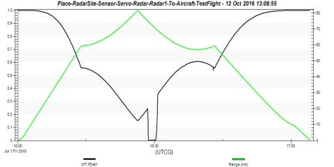
PDet Range Graph
You are looking for a PDet of 0.5 or greater. It's a given that as distance increases, your PDet will decrease. There are instances where your tracking drops well below a PDet of 0.5. Using the Toggle animation time line button, right clicking on the graph, and selecting Set Animation Time, enables you to jump back to the 3D Graphics window to visualize what is occurring. In the following picture, you can see that the UAV is flying behind a mountain based on the time line shown in the PDet Range Graph.
Overall, the radar system is able to track the UAV. It's time to see if you can jam the radar.
Radar Jamming
You will simulate an aerostat flying near Mount St. Helens. The aerostat is tethered at 10000 feet AGL.
- Insert a Place () object using the Define Properties method. .
- On the Basic - Position page, make the following changes:
- Click OK.
- Rename the Place object "JamSite".
| Option | Value |
|---|---|
| Latitude | 46.1173 deg |
| Longitude | -122.315 deg |
| Height Above Ground | 10000 ft |
The Jammer
You can model the radar jammer by simply reusing the previously built surveillance radar and making a couple of changes. You'll use some specifications from the AN/ALQ-99 Tactical Jamming System (TJS).
- In the Object Browser, copy Servo and paste it to JamSite.
- Rename JamSite's Radar object "Jammer".
- Open JamSite's sensor's () properties ().
- Browse to the Basic - Location page and change the Location Type to Center.
- Browse to the Basic - Pointing page.
- Remove TestFlightfrom the Assigned Targets list and replace it with RadarSite..
- Click OK.
- Rename JamSite's Radar object "Jammer".
- Return to the 3D Graphics window and Zoom To JamSite.
Define the Jammer
JamSite is at 10000 feet AGL. The Sensor object is attached to JamSite's center and is targeting RadarSite.. Make the required specification changes to the jammer using a couple TJS specifications.
- Open Jammer's () properties ().
- On the Basic - Definition page, select the Antenna tab and change the Type to Square Horn.
- Change the Diameter to 1ft (one foot).
- Select the Transmitter tab.
- Change the Power to 10.8 kW.
- Click OK.
Jam the Radar
The next step is to tell the surveillance radar that it's being jammed.
- Open the surveillance Radar () properties ().
- On the Basic - Definition page, select the Jamming tab.
- Enable Use and move the jam Radar object to the Assigned Jammers field.
- Click OK.
You are now ready to analyze Jammer's effectiveness against the surveillance radar.
Jam Effectiveness
Create a custom graph that shows only those contents you are interested in for your analysis. You are interested in S/T PDet1 (Search/Track Probability of detection) and S/T PDet1 w/ Jamming (Search/Track Probability of detection with jamming).
- In the Object Browser, right click on the surveillance Radar () and open the Access () tool.
- In the Associated Objects List, select TestFlight.
- Click the Report & Graph Manager... button.
- Select the My Styles folder and click the Create new graph style button.
- Give the graph a name such as PDet Jamming then click the Enter key on your keyboard.
- In the Data Provider window, expand Radar Search Track.
- Move (
 ) S/T PDet1 to the Y Axis window.
 - Move () the S/T PDet1 w/ Jamming to the Y Axis window.
- Click OK.
- Generate the graph.
By placing the Pdet and Pdet with jamming on the same axis, it's easier to read the graph. As you can see by looking at the graphthe jammer attached to the aerostat is effectively jamming the surveillance radar.
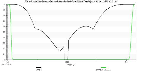
PDet With Jamming
Don't forget to save your work!
 Visit AGI.com