STK Professional and Communications.
The results of the tutorial may vary depending on the user settings and data enabled (online operations, terrain server, dynamic Earth data, etc.). It is acceptable to have different results.
This walkthrough introduces you to some of the 2D and 3D graphics capabilities available in STK Communications. In this exercise you will:
- Define and display contours of antenna gain and other RF characteristics in the 2D and 3D Graphics windows
- Use vectors to enhance the 3D Graphics window display of a transmitter on a GEO satellite
- Create and vary 3D Graphics window representations of antenna beam patterns
Create a Scenario
Start by creating a scenario.
- Create a scenario and name it CommGraphics.
- Set the Start time to 1 Jul 2016 18:00:00.000 UTCG.
- Set the Stop time to 2 Jul 2016 18:00:00.000 UTCG.
Save Often!
Add a Satellite
For the communications satellite, you'll use the Orbit Wizard to create a geosynchronous satellite.
- Using the Insert STK Objects tool, insert a Satellite object using the Orbit Wizard method.
- When the Orbit Wizard window appears, make the following changes:
- Click OK.
| Option | Value |
|---|---|
| Type: | Geosynchronous |
| Satellite | CommSat |
Add a Receiver
- Using the Insert STK Objects tool, insert a Receiver (
 ) object using the Insert Default method.
 - When the Select Object window appears, select CommSat and then click OK.
- In the Object Browser, rename the Receiver object "CommRcvr."
- Open CommRcvr's () properties (
 ).
). - On the Basic - Definition page, change Type: to Complex Receiver Model.
- Click Apply.
- Select the Antenna tab.
- Note that the Main-lobe Gain: is approximately ~ 41 dB.
The default antenna for a Complex Receiver Model is Gaussian. The satellite that the antenna is attached to is in a Geosynchronous orbit. The orientation of the antenna is azimuth 0 degrees and elevation is 90 degrees. Therefore, the main-lobe gain is directed along the Satellite objects Z body which is pointing towards nadir.
Communication Contours
- Browse to CommRcvr's () 2D Graphics - Contours page.
- Enable Show Contour Graphics.
- Disable Relative To Maximum.
- In the Level Adding field, change Add Method: to Explicit.
- Change the Level: value to 41 (the approximate maximum gain for this antenna in dB).
- Click the Add Level button which adds it to the Level Attributes field.
- Repeat steps 4 and 5 to add the following gain levels to the Level Attributes field: 30, 20, 10, 0, -10, and -20.
- In the Level Labels: field, enable Show and set Number of Decibel Digits to 0.
- Ensure Color Method is set to Color Ramp.
- Set Start Color: to Red and Stop Color: to Blue.
- Click Apply.
View the Contours
You can view the contour graphics in the 2D Graphics window.
- Bring the 2D Graphics window to the front.
- Mouse around in the 2D Graphics to view the contours.
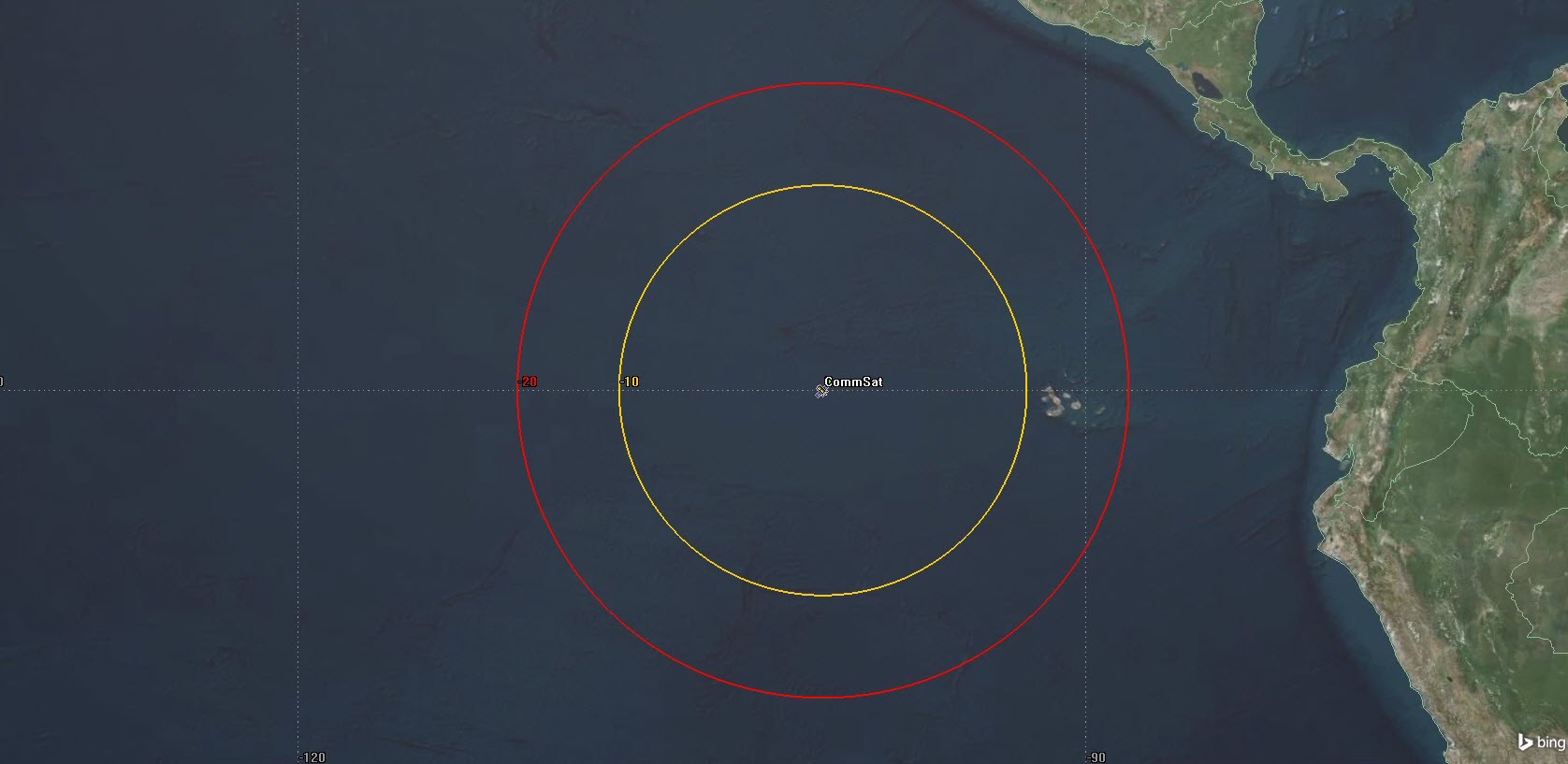
Receiver Contours
Using this method, each contour is the actual main-lobe gain value of the receiver's antenna.
Saving Time and Effort
There are two options that can simplify and speed up the generation of gain contours:
- Use the Relative to Maximum option instead of retrieving the maximum gain value from the Antenna Parameters
- Use Start, Stop, Step as the Add Method instead of manually entering each gain level
Run through the above process again, using these convenient options.
- Return to CommRcvr's () properties and select the 2D Graphics - Contours page.
- Enable Relative To Maximum.
- In the Level Attributes field, click the Remove All button.
- In the Level Attributes field, make the following changes:
- Click the Add Level button.
- Click Apply.
- Return to the 2D Graphics window to view the new contours.
| Option | Value |
|---|---|
| Add Method: | Start, Stop, Step |
| Start | 0 |
| Stop | -60 |
| Step | -10 |
A value of 0 relative to maximum is equivalent to the maximum gain value, i.e. approximately 41 dB. A value of -10 is 10 dB less than the maximum.
On Your Own
Before leaving receiver antenna gain contours, try some other options that are provided on the Contours page. After each change, click Apply on the Contours page, and return to the 2D Graphics window.
- Change the Add Method to Explicit, and add a new level of -35 dB to the Level list.
- Select one or more entries from the Level list, and change the Line Style (e.g. to dotted or dashed).
- Change the Line Width for all gain levels to a different thickness.
- Select the Show at Altitude option, and enter an Altitude value of 5000 km. Instead of representing gain levels where the antenna beam intersects the Earth’s surface (the normal case), the contour pattern now represents gain levels where the beam crosses the selected altitude. When you reset the 2D Graphics window, the contour pattern will noticeably contract.
- When finished, disable Show Contour Graphics.
- Click OK.
Line Style settings apply only to levels that you select.
Line Width settings always apply to all contour levels in the pattern.
Receiver object contour graphics are available only for Antenna Gain.
Add a Multibeam Transmitter
- Using the Insert STK Objects tool, insert a Transmitter (
 ) object using the Insert Default method.
 - When the Select Object window appears, select CommSat (
 ) and then click OK.
 - In the Object Browser, rename the Transmitter object "MultibeamXmtr".
- Open MultibeamXmtr's () properties ().
- On the Basic - Definition page, change Type: to Multibeam Transmitter Model.
- In the Beams tab, click the Add button to insert two more beams.
- Click Apply.
Re-orient the Beams
- Using the Shift key, select all three beams.
- Click the Orient button.
- In the Antenna Beam Orientation window, make the following changes to the Elevation Initial State and the Azimuth Increment value:
| Antenna Beam Orientation | Initial Value | Increment Value |
|---|---|---|
| Elevation | 87 deg | 0 deg |
| Azimuth | 0 deg | 120 deg |
- Click OK to close the Antenna Beam Orientation window.
- Click Apply.
Communication Contours
- Browse to MultibeamXmtr's () 2D Graphics - Contours page.
- Enable Show Contour Graphics.
- Change Type: to EIRP (Effective Isotropic Radiated Power).
- In the Level Adding field, make the following changes:
- Click the Add Level button.
- In the Level Labels: field, enable Show and set Number of Decibel Digits to 0.
- Ensure Color Method is set to Color Ramp.
- Set Start Color: to Red and Stop Color: to Blue.
- Click Apply.
- Return to the 2D Graphics window to view the new contours.
| Option | Value |
|---|---|
| Add Method: | Start, Stop, Step |
| Start | 0 |
| Stop | -60 |
| Step | -10 |
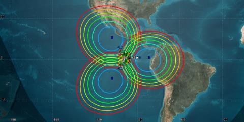
Max Gain Beams
Change Beam Selection Strategy
The current beam selection strategy is Max Gain.
- Return to MultibeamXmtr's () properties and browse to the Basic - Definition page.
- Change Beam Selection Strategy to Aggregate Active Beams.
Combines gains to model a single beam with a gain aggregating the gains of all individual beams. The beam powers are also combined with the respective gains to compute the aggregate EIRP for the antenna.
- Click Apply.
- Return to the 2D Graphics window to view the new contours.
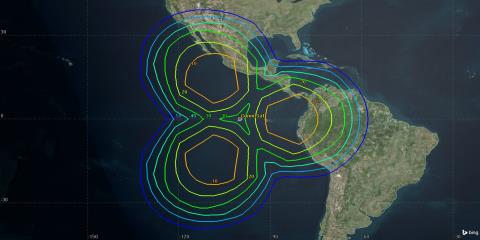
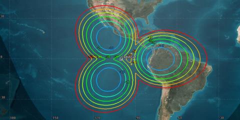
Aggregate Active Beams
Improve Resolution
You can improve the resolution of the contours.
- Browse to MultibeamXmtr's () 2D Graphics - Contours page.
- Enable Set azimuth and elevation resolution together.
- In the Azimuth field, change the Resolution value to 0.5 deg.
- Click Apply.
- Return to the 2D Graphics window to view the new contours.
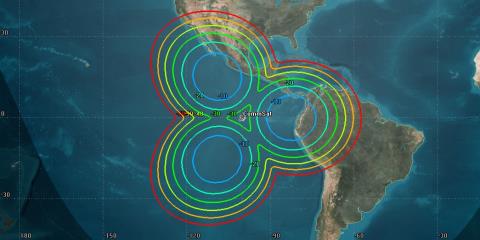
Enhanced Contours
There should be a noticeable change in the resolution of the contour graphics.
In MultibeamXmtr's (![]() ) 2D Graphics - Contours page, the Points field, immediately below the Resolution field, will automatically update to reflect the finer resolution value.
) 2D Graphics - Contours page, the Points field, immediately below the Resolution field, will automatically update to reflect the finer resolution value.
Contours in 3D
Contours can also be displayed in the 3D Graphics window.
- Browse to MultibeamXmtr's () 3D Graphics - Attributes page.
- In the Contour Graphics field, enable Show Lines.
- Click Apply.
- Select the 3D Graphics window to view the new contours.
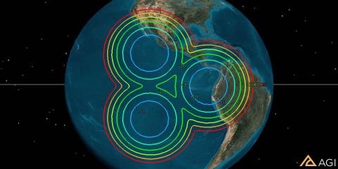
3D Graphics Contours
Reorient One Antenna
- Return to MultibeamXmtr's () properties and browse to the Basic - Definition page.
- Select the Antenna tab.
- Select the Orientation tab.
- In the Position Offset field, change the X value to 1000 km.
- Click Apply.
- Select the 2D Graphics window to view the new contours.
- After viewing the effect of the offset on the contour graphics, return to the Position Offset field and reset the X value to zero (0) m.
- Click Apply.
Orientation Change
In addition to EIRP, transmitter contour graphics are available for Antenna Gain, Flux Density, and RIP (Received Isotropic Power). Before moving on in the tutorial, try out one or more of the contour types using the Relative to Maximum option and the Start, Stop, Step method to avoid having to determine or guess absolute values.
Unlike Antenna Gain, which can be retrieved directly from the Antenna properties, determination of appropriate values for the other contour types requires creating additional objects, calculating access, and generating link budget reports.
Disable the Contour Graphics
Let's clean up the 3D Graphics window of the contour graphics. This way you can continue on with creating vectors and the contour graphics won't impede your view.
- When you are finished experimenting, return to MultibeamXmtr's properties and browse to the 2D Graphics - Contours page.
- Disable Show Contour Graphics.
- Browse to the 3D Graphics - Attributes page.
- In the Contour Graphics field, disable Show Lines.
- Click OK.
Enhance the 3D Display with Vectors
In the following exercise you will:
- Configure the Satellite object and the Transmitter object to display body axes
- Attach the Transmitter object to a Sensor object and set the Sensor object spinning
- Observe the display of the Satellite and Transmitter objects axes in the 3D Graphics window
- Open CommSat's () properties and browse to the 3D Graphics - Vector page.
- Select the Axes tab.
- Enable Body Axes - Show.
- Change the color if desired by double clicking on the color pane. This provides a pull-down menu which allows you to choose a new color.
- Click OK.
- In the Object Browser, right click on CommSat () and select Zoom To.
- Select the 3D Graphics window.
- Zoom and rotate the 3D view, as necessary, to see the axes.
Satellite Body Axis
Add a Sensor
- Using the Insert STK Objects tool, insert a Sensor (
 ) object using the Insert Default method.
 - When the Select Object window appears, select CommSat () and then click OK.
- In the Object Browser, rename the Sensor object "SatSens".
- Open SatSens's () properties (), and browse to the Basic - Pointing page.
- Change Pointing Type: to Spinning.
- In the Spinning field, change the Spin Rate value to .2 revs/min.
- Browse to the 3D Graphics - Attributes page.
- In the Lines field, enable Translucent Lines.
- In the Projection field, change the %Translucency: value to 100.
- Click OK.
The translucency is increased so that display of the sensor cone in the 3D Graphics window does not interfere with display of the vector graphics.
Reusing Objects
- In the Object Browser, right-click on MultibeamXmtr () and select Cut (
 ) from the Edit menu.
 - Right-click on SatSens () and select Paste (
 ) from the Edit menu.
 - Expand SatSens so that you can see MultibeamXmtr.
Cut and paste is an easy way to move objects around in the scenario hierarchy. You can also use copy-and-paste to create duplicates of objects that you have previously created and configured. When you move or copy an object that has sub-objects, the sub-objects are moved or copied along with their parent object.
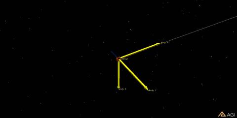
Display the Transmitter's Body Axis
- Open MultibeamXmtr's () properties ().
- Browse to the 3D Graphics - Vector page.
- Select the Axes tab.
- Enable Body Axes - Show.
- If desired, change the color to a different color being used by the parent object's body axis.
- Click Apply.
- Zoom To CommSat ().
- Bring the 3D Graphics window to the front.
![]()
Transmitter Body Axis
Animate the Scenario
Let's take a look at the body axes in motion.
- Using the Decrease Time Step (
 ) button in the Animation toolbar, decrease the time step to 1.0 Sec.
 - Using the Start button in the Animation toolbar, briefly animate the scenario to observe the transmitter body axes as they rotate with respect to the satellite body axes in the 3D Graphics window.
- When finished, click the Reset (
 ) button in the Animation toolbar to reset the scenario back to the Start time.
The Sensor object "acted" as a motor to move the antenna.
Sun Vector
- Return to MultibeamXmtr's () properties () and browse to the 3D Graphics - Vector page.
- Select the Vectors tab and enable Sun Vector - Show.
- Click Apply.
- Return to the 3D Graphics window.
- Using the Start (
 ) button in the Animation toolbar, briefly animate the scenario to observe the transmitter body axes and sun vector as they rotate with respect to the satellite body axes in the 3D Graphics window.
 - When finished, click the Reset () button in the Animation toolbar to reset the scenario back to the Start time.
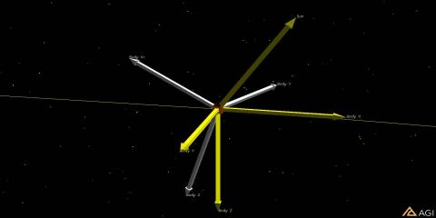
Sun Vector
A representative selection of vectors and axes is listed on MultibeamXmtr's 3D Graphics - Vector properties page, but you are by no means limited to those. Click Add… to browse through the large variety of vectors, axes, and other components that you can add to your 3D display.
Before moving on to antenna beam patterns, experiment with other graphics settings on MultibeamXmtr’s Vector page, or click Add… and introduce other components into your 3D display.
Disable the Vectors
- When finished, return to MultibeamXmtr's () properties 3D Graphics - Vector page.
- Select the Axes tab.
- Disable Body Axes - Show.
- Select the Vectors tab.
- Disable Sun Vector - Show.
- Disable any components you may have added.
- Click OK.
- Open CommSat's () properties ().
- Browse to the 3D Graphics - Vector page.
- Select the Axes tab.
- Disable Body Axes Show.
- Click OK.
Antenna Beam Patterns
To display the shape and gain levels of antenna beams you can use Volume Graphics.
- In the Object Browser, Cut () MultibeamXmtr () from SatSens () and Paste () it to CommSat ().
- Open MultibeamXmtr's () properties ().
- Browse to the 3D Graphics - Attributes page.
- In the Volume Graphics field, enable Show Volume.
- Change the Gain Scale (per dB) value to 800 km.
- Enable Set azimuth and elevation resolution together.
- Change the Azimuth - Resolution value to 0.5 deg.
- Click Apply.
View the Beam Patterns in 3D
- Bring the 3D Graphics window to the front.
- Click the Home View button in the 3D Graphics window toolbar.
- Use your mouse to manipulate your view so that you can see the Volume Graphics of the multibeam antenna pattern.
- To add contour graphics back into the 3D view, return to the MultibeamXmtr's 3D Graphics - Attributes page, check Show Lines in the Contour Graphics field, and click Apply.
- You can also bring the MultibeamXmtr’s body axes back into the picture which is found at the 3D Graphics - Vector page. For better display, increase the Scale to 6.0.
- When finished, return to MultibeamXmtr's () properties ()and click OK.
- Go to the Object Browser and disable MultibeamXmtr ().
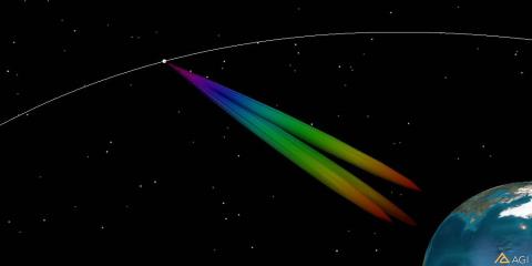
Volume Graphics
The colors of the beam pattern represent gain levels, running the spectrum from red (relatively high gain) to violet (relatively low gain). The size of the beam pattern is determined by the setting for Gain Scale (see above), which specifies the number of kilometers per dB of gain.
Receiver Volume Graphics
- Open CommRcvr's () properties ().
- On the Basic - Definition page, disable Frequency: Auto Track.
- Change the Frequency: value to 2.5 GHz.
- Select the Antenna tab.
- In the Model Specs tab, make the following changes:
- Click Apply.
- Browse to the 3D Graphics - Attributes page.
- In the Volume Graphics field, enable Show Volume.
- In the Azimuth field, change the Resolution value to 1 deg.
- In the Elevation field, change the Resolution to 1 deg.
- Click Apply.
| Option | Value |
|---|---|
| Type: | Helix |
| Diameter: | .1 m |
View in the 3D Graphics Window
- Bring the 3D Graphics window to the front.
- Zoom To CommSat ().
- Use your mouse to manipulate the view so that you have a good view of CommRcvr's Volume Graphics.
- Return to CommRcvr's () properties ().
- On the 3D Graphics - Attributes page, in the Volume Graphics field, enable Show as wireframe.
- Click Apply.
- Return to the 3D Graphics window.
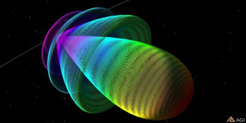
Wireframe Mode
This exercise illustrates only a few of the things you can do with antenna beam patterns. Experiment with other Definition settings (e.g. frequency, antenna model, antenna size) and graphics options. Observe the results in the 3D Graphics window.
 Visit AGI.com