STK Professional, Communications, Coverage and Analysis Workbench.
The results of the tutorial may vary depending on the user settings and data enabled (online operations, terrain server, dynamic Earth data, etc.). It is acceptable to have different results.
Using the STK Communications module, access between a transmitter and a receiver can be constrained to satisfy a variety of RF criteria. With one or more constraints in place, you can adjust the properties of the communications devices and see how the adjustments affect link performance. In the following exercise, you will set up a link between a ground‐based receiver and a transmitter on a communications satellite, then impose various communication constraints and observe the effects.
Create a Scenario
Start by creating a scenario.
- Create a scenario (
 ) and name it Comm_Constraints.
 - Change Start: to 1 Jul 2016 16:00:00.000 UTCG and Stop: to + 24 hrs.
Save Often!
Radio Frequency (RF) Environment
Before defining parameters that are specific to the transmitter and receiver, it will be useful to select environmental models applicable to any communications link in the scenario.
- Open the scenario's () properties (
 ).
). - Browse to the Basic – Terrain page.
- Disable Use terrain server for analysis.
- Browse to the
- Select the Rain & Cloud & Fog tab.
- In the Rain Model field, enable Use.
- Select the available ITU (International Telecommunications Union) model.
- Select the Atmospheric Absorption tab.
- Enable Use.
- Select the available ITU model.
- Click OK.
Insert a Ground Station
Use a Facility object from the Standard Object Database that is located in the central portion of the United States.
- Using the Insert STK Objects tool, insert a Facility (
 ) object using the
 - Enter Offutt in the Name: option.
- Click Search.
- Select Offutt AFB SATCOM Terminal in the Search Results field.
- Click Insert.
- Close the Search Standard Object Data window.
Insert a Satellite
Add a new Satellite object to the scenario using the Orbit Wizard.
- Using the Insert STK Objects tool, insert a Satellite (
 ) object using the Orbit Wizard (
 ) method.
 - Change Satellite to "CommSat."
- In the Definition field, change Altitude: to 1500 km.
- Leave the remaining default settings and click OK.
Communication Equipment
In this scenario, you will have a Transmitter object attached to the Satellite object that is used to downlink information to the Facility object. The Facility object will have a Receiver object that receives the downlink transmission. Both the Receiver and Transmitter objects can be targeted. In STK, you will use a Sensor object as the targeting device.
Satellite Pointing Device
- Using the Insert STK Objects tool, insert a Sensor (
 ) object using the Insert Default method.
 - When the Select Object window appears, select CommSat and then click OK.
- In the Object Browser, rename the Sensor object "TgtOffutt."
- Open TgtOffutt's () properties ().
- On the Basic - Definition page, in the Simple Conic field, change Cone Half Angle: to two (2) deg. This is for situational awareness only.
- Browse to the Basic - Pointing page.
- Set the Pointing Type to Targeted.
- Move (
 ) Offutt_AFB_SATCOM_Terminal from the Available Targets list to the Assigned Targets list using the right arrow.
 - Click OK.
Downlink Transmitter
Use a Complex Transmitter as the downlink transmitter.
- Using the Insert STK Objects tool, insert a Transmitter (
 ) object using the Insert Default method.
 - When the Select Object window appears, select TgtOffut and then click OK.
- In the Object Browser, rename the Transmitter object "DLXmtr."
- Open DLXmtr's () properties ().
- On the Basic - Definition page, make the following changes:
- Click OK.
| Option | Value |
|---|---|
| Type: | Complex Transmitter Model |
| Frequency: | 4.5 GHz |
| Power | 5 dBW |
Downlink Receiver
Use a Medium Receiver Model as the downlink receiver.
- Using the Insert STK Objects tool, insert a Receiver (
 ) object using the Insert Default method.
 - When the Select Object window appears, select Offutt_AFB_SATCOM_Terminal and then click OK.
- In the Object Browser, rename the Receiver object "DLRcvr."
- Open DLRcvr's () properties ().
- On the Basic - Definition page, make the following changes:
- Click Apply.
| Option | Value |
|---|---|
| Type: | Medium Receiver Model |
| Gain: | 20 dB |
| Rain Model - Outage Percent | 0.010 |
The Outage Percentage expresses as a percentage how much time can be sacrificed to rain outage during the year or, conversely, how much time the link must be maintained despite rain. In this case you are specifying that the link must be maintained 99.99 percent of the year, rain or no rain, and other parameters, such as power or frequency, may need to be adjusted to meet this requirement.
Set the System Noise Temperature
- Select the System Noise Temperature tab.
- Select the Compute option.
- In the LNA field, set the Noise Figure to 1.2 dB.
- In the Antenna Noise field, enable Compute.
- Enable the Sun, Atmosphere, and Rain options.
- Click Apply.
Model Atmospheric Refraction
Atmospheric refraction is the bending of an RF signal as it travels through the atmosphere, caused by the changing refractive index at different altitudes.
- Select the Basic - Refraction page.
- Enable Use Refraction in Access Computations.
- Change Refraction Model: to the available ITU model.
- Click OK.
This model computes the refracted elevation on the basis of inputs consisting of the non‐refracted elevation angle and the mean sea level altitude of the receiver, using empirical criteria contained in ITU Recommendation. This completes the setup of the receiver.
Calculate Access
A Link Budget can now be calculated between DLXmtr and DLRcvr. Let's determine if the receiver can talk to the transmitter.
- In the Object Browser, right click on DLRcvr () and select Access (
 ).
). - When the Access Tool opens, in the Associate Objects list, expand (
 )CommSat (), then TgtOffutt (), and select DLXmtr ().
 - Click Compute.
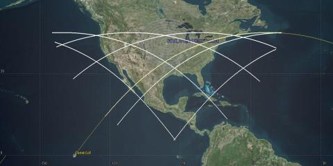
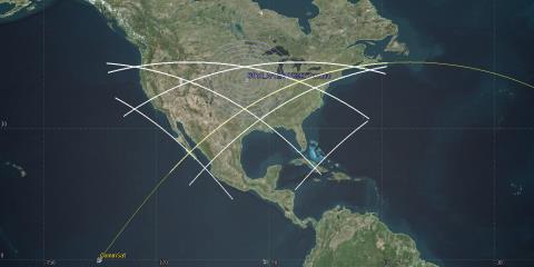
- Bring the 2D Graphics window to the front.
Access highlights in the 2D visualization window will show portions of the satellite's ground track where there is access between the transmitter and receiver.
Clean Compute
In the remainder of this exercise, when communication constraints are imposed that limit the periods of access on the basis of given RF criteria, it will be interesting to observe corresponding changes in the access graphics.
Generate a Link Budget Report
- Return to the Access Tool () and click the Report & Graph Manager... button.
- When the Report & Graph Manager opens, in the Styles field, expand () Installed Styles directory.
- Select the Link Budget - Detailed report.
- Click Generate.
Constraints
With the report open, you can change communication constraints and refresh the report to see the effects your constraints create on the link performance.
Received Isotropic Power Constraint
In the Link Budget - Detailed report, take a look at the values for Received Isotropic Power (RIP), which is the product of the Effective Isotropic Radiated Power (EIRP) of the transmitter and the propagation (atmospheric, rain, and free space losses) without any contribution by the receiver. These values fall in the approximate range of ~ –149 to -133 dBW, according to the Link Budget Report.
Suppose it is desirable to exclude any link with an RIP value of less than –140 dBW.
- Open DLRcvr's () properties ().
- Browse to the Constraints - Comm page.
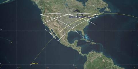
- In the Rcvd Isotropic Power field, enable Min: and set the value to -140 dBW.
- Click Apply. In the 2D visualization window, you will see that the constraint you imposed has a significant impact on access times.
- Return to the Link Budget - Detailed report.
- Click the Refresh button.
RIP Constraint
Disable the RIP Constraint
No time entries for RIP values less than –140 dBW will appear in the report.
- Return to DLRcvr's () properties ().
- Browse to the Constraints - Comm page.
- In the Rcvd Isotropic Power field, disable Min.
- Click Apply.
- Return to the Link Budget - Detailed report and click the Refresh button.
Doppler Shift Constraint
The Doppler Shift constraint relates to the ability of the receiver to adjust to increases in the frequency of the incoming signal as the satellite approaches its closest point to the receiver and to adjust to decreases in that frequency as the satellite moves away from that point. Recall you specified a transmitter frequency of 4.5 GHz. If you now look at the figures for Received Frequency in the Link Budget Report (refresh it if necessary, and make certain that all constraints are removed), you will see that the receiver must accommodate a shift of about +/‐81 kHz in frequency to avoid losing any of the incoming signal.
Suppose the receiver is limited to a 50 kHz adjustment in either direction.
- Return to DLRcvr's () properties () and browse to the Constraints - Comm page.
- In the Doppler Shift field, enable both Min: and Max:.
- Set Min: to -50 kHz.
- Set Max: to 50 kHz.
- Click Apply.
- Return to the Link Budget - Detailed report and click the Refresh button.
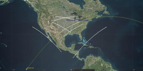
- Bring to 2D Graphics window to the front.
You will notice that time entries for Received Frequencies less than 4.499950 GHz and greater than 4.500050 GHz are excluded.
Doppler Constraint
Disable the Min and Max Doppler Shift Constraints
The 2D visualization window will clearly reflect the impact of this constraint. In fact, if you alternatively disable and enable the Min and Max options, you will see that the Doppler shift limitations are reflected alternatively in the approaching and departing ground tracks, just as you would expect.
- Return to DLRcvr's () properties () and browse to the Constraints - Comm page.
- In the Doppler Shift field, disable both Min: and Max:.
- Click Apply.
- Return to the Link Budget - Detailed report and click the Refresh button.
Flux Density Constraint
Flux Density, usually measured in dB (watts/m^2), is the expression of the transmitter's radiated power (reduced by any applicable atmospheric losses) divided by the surface area of a sphere whose radius equals the distance between the transmitter and receiver:
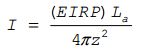
Flux Density
In the Link Budget - Detailed report, entries for Flux Density should range between approximately -114 and –99 dBW/m^2. Now suppose you wish to exclude from consideration links with a Flux Density less than –110 dBW/m^2.
- Return to DLRcvr's () properties () and browse to the Constraints - Comm page.
- In the Flux Density field, enable Min:.
- Set Min: to -110 dBW/m^2.
- Click Apply.
- Return to the Link Budget - Detailed report and click the Refresh button. You will notice that time entries for Flux Density less than -110 dBW/m^2 are excluded.
- Bring to 2D Graphics window to the front.

2D Flux Density
The 2D Graphics view didn't change very much due to the loss of just a few time entries.
Disable the Constraint
- Return to DLRcvr's () properties () and browse to the Constraints - Comm page.
- In the Flux Density field, disable Min:.
- Click Apply.
- Return to the Link Budget - Detailed report and click the Refresh button.
Carrier to Noise Ratio Constraints
One of the most commonly used criteria for assessing link performance is Carrier to Noise Ratio (CNR). This can be expressed independently of bandwidth as:
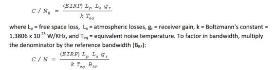
CNR Expression
For the communications link in this exercise, C/No and C/N fall in the approximate ranges 74 to 95 dB/Hz and ‐1 to 20 dB, respectively. You can constrain link performance with respect to either of these criteria. Now suppose you wish to exclude from consideration links with a Carrier to Noise Ratio of less than 10 dB.
- Return to DLRcvr's () properties () and browse to the Constraints - Comm page.
- In the C/N field, enable Min:.
- Set Min: to ten (10) dB.
- Click Apply.
- Return to the Link Budget - Detailed report and click the Refresh button. You will notice that time entries for C/N less than ten (10) dB are excluded.
- Bring to 2D Graphics window to the front.
CN Constraint
Reset the Receiver's Properties
C/No and C/N can be improved via receiver as well as transmitter adjustments, since receiver gain appears in the numerator both equations. Leave the C/N constraint in place, and from the receiver’s Basic – Definition page, try each of the following adjustments one at a time – resetting each parameter to its original value before proceeding to the next.
- Return to DLRcvr's () properties () and browse to the Basic - Definition page.
- In the Model Specs tab, increase Gain to 25 dB.
- Click Apply.
- Return to the Link Budget - Detailed report and click the Refresh button.
- Note the changes in the C/No and C/N field.
- Return to DLRcvr's () properties () and browse to the Basic - Definition page.
- In the Model Specs tab, decrease the Gain to 20 dB.
- Click Apply.
- Return to the Link Budget - Detailed report and click the Refresh button.
Your settings are back to the original settings. Continue with the remaining steps one at a time – resetting each parameter to its original value before proceeding to the next like you did in steps one (1) through nine (9).
- On the System Noise Temperature tab, reduce LNA Noise Figure to one (1) dB.
- On the Model Specs tab, add (Right Hand or Left Hand) Circular Polarization. You must also set the polarization on the transmitter to the same type.
- On the Additional Gains and Losses tab, add a Pre‐Receive gain of one (1) dB.
- On the Model Specs tab, increase the Rain Model Outage Percent to 0.030.
At this point, Rain Model Outage should be back at 0.010 and the only Comm Constraint that is enabled is C/N. Everything else should be reset.
Disable the Constraints
- Return to DLRcvr's () properties () and browse to the Constraints- Comm page.
- Remove all constraints.
- Click OK.
- Return to the Link Budget - Detailed report and click the Refresh button.
Modulation Adjustment
An interesting transmitter adjustment to try out is a change in the Modulation Type.
- Open DLXmtr's () properties () and browse to the Basic - Definition page.
- Select the Modulator tab.
- Set the Name to MSK.
- Click Apply.
- Return to the Link Budget - Detailed report and click the Refresh button.
From here on in, you can keep going back to the 2D Graphics window to see the constraint effects on access times.
Set the Modulation back to BPSK
In digital modulation, minimum-shift keying (MSK) is a type of continuous-phase frequency-shift keying. The default modulation in STK is binary phase-shift keying (BPSK).
- Return to DLXmtr's () properties () and browse to the Basic - Definition page.
- Select the Modulator tab and change Name back to BPSK.
- Click Apply.
- Return to the Link Budget - Detailed report and click the Refresh button.
Constraints on Digital Systems
For digital communications systems, the receiver bit energy to noise ratio is defined as:
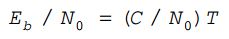
Digital System Definition
where T = the bit period. As reflected in the Link Budget report the communications link in this exercise exhibits Eb/No values ranging from approximately two (2) to 23 dB.
Energy Per Bit to Noise Power Spectral Density Ratio or Eb/No Constraints
- Return to DLXmtr's () properties () and browse to the Basic - Definition page.
- In the Model Specs tab, change Data Rate: to 12 Mb/sec.
- Click Apply.
- Browse to the Constraints - Comm page.
- In the Eb/No field, enable Min:.
- Change Min: to 15 db.
- Click Apply.
- Return to the Link Budget - Detailed report and click the Refresh button.
As with CNR, link performance can be improved by tweaking receiver or transmitter parameters. This increases the bit period T, which leads directly to an improvement in Eb/No.
Disable the Constraint
- Return to DLXmtr's () properties () and browse to the Constraints - Comm page.
- In the Eb/No field, disable Min:.
- Click Apply.
- Browse to the Basic - Definition page.
- Change Data Rate: back to 16 Mb/sec.
- Click Apply.
- Return to the Link Budget - Detailed report and click the Refresh button.
Bit Error Rate Constraints
A direct measure of link performance for a digital system is Bit Error Rate (BER), which expresses the probability that a bit will be received in error. According to the Link Budget report, BER values in this exercise range from approximately 1 x 10‐30 to 4.5 x 10‐2. A typical desired BER is 10‐6.
- Return to DLXmtr's () properties () and browse to the Constraints - Comm page.
- In the Bit Error Rate field, enable Max:.
- Change Max: to 1e-006.
- Click Apply.
- Return to the Link Budget - Detailed report and click the Refresh button.
BER is a function of Eb/No, and you can improve it through adjustments in the receiver or transmitter, including reductions in Data Rate.
Disable the Constraint
- Return to DLXmtr's () properties () and browse to the Constraints - Comm page.
- In the Bit Error Rate field, disable Max.
- Click OK.
- Return to the Link Budget - Detailed report and click the Refresh button.
Refracted Elevation and Range Constraints
Constraints can be set in terms of the refracted elevation and range of the transmitter with respect to the receiver. As a reminder, you are currently using the ITU refraction model in your analysis.
Elevation Angle Constraint
- Open DLRcvr's () properties ().
- Browse to the Constraints - Basic page.
- In the Elevation Angle field, enable Min.
- Set the Min to five (5) deg.
- Click Apply.
- Return to the Link Budget - Detailed report and click the Refresh button.
This excludes links with satellites deemed to be too close to the horizon, which can be unreliable due to the relatively long path through the atmosphere to be traversed by the signal. You'll notice in the Link Budget - Detailed report, most if not all of your BER fall within acceptable range (at or below 1 x 10‐6).
Refraction Angle
The calculation of the refracted elevation or range depends on the selected refraction model. As you may recall, you selected an ITU model satisfying empirical criteria.
- Return to DLRcvr's () properties () and browser to the Basic - Refraction page.
- Change Refraction Model to Effective Radius Method. This computes the apparent elevation due to refraction.
- Click Apply.
- Return to the Link Budget - Detailed report and click the Refresh button.
You will see improved Eb/No and BER values. Using this model, the 2D Graphics window should reflect a marginally larger portion of the satellite's orbit satisfying the elevation constraint than under the more empirically grounded ITU model. When “Use Refraction in Access Computations” is enabled, object visibility, range, elevation angle, and link angle of the antenna boresight are computed with refraction taken into account.
An Everyday Use of C/N Constraints
It is a common practice for a receiver vendor to stipulate a minimum required C/N value that must be satisfied in order for its equipment to perform to specification. Imposing a C/N constraint on accesses between a receiver and a transmitter is an easy way to model this requirement in the design of communications links. For example, if the manufacturer specifies that its equipment requires a C/N value of at least five (5) dB to function properly, you can simply enter a Min value of five (5) for the C/N constraint, which will reduce the number and/or length of calculated periods of access between the receiver and transmitter.
For greater confidence in the quality and reliability of a link, it is a good idea to add a fade margin to other requirements that must be met. A natural way to do this is to increase the Min value of the C/N constraint to include that margin. Thus, to model a fade margin of three (3) dB for a receiver requiring a minimum C/N value of five (5) dB, just set the Min value for C/N to eight (8) dB. You can then enjoy a higher degree of confidence in the access periods.
- Prior to moving on to the next section, place all properties back to their original settings.
- Close the report, Report & Graph Manager, Access Tool, and any object properties.
Using Communication Constraints in Coverage
You can use the Coverage Definition object to analyze a portion of a link budget (i.e. C/N) over a wide area. Communication constraints will affect the coverage.
Insert an Area Target
The Area Target object models a region on the surface of the central body.
- Insert an Area Target object using the Select Countries and US States method.
- Disable the US States option in the List Selections field.
- Select United_States in the list.
- Click Insert.
- Click Close.
Insert a Coverage Definition Object
- Insert a Coverage Definition object using the Insert Default method.
- Open the Coverage Definition object’s properties.
- Select the Basic – Grid page.
Coverage analyses are based on the accessibility of assets (objects that provide coverage) and geographical areas. For analyses purposes, the geographical areas of interest are further refined using regions and points.
- In the Grid Area of Interest field, change Type: to Custom Regions.
- Click the Select Regions button.
- Move United_States to the Selected Regions list.
- Click OK to accept the changes to the Select Regions window.
The statistical data computed during a coverage analysis is based on a set of locations, or points, which span the specified grid area of interest.
- In the Grid Definition field, set the Point Granularity to two (2) degrees.
Once you have defined the grid area, you can specify an object class or a specific object for the points within the grid. The object can be used to associate three types of information with the grid points: access constraints, basic object properties, and the shape of the ellipsoidal obstruction surface used by the Line Of Sight constraint.
- Click the Grid Constraints Options... button.
- Set the Reference Constraint Class to Receiver.
- Select Offutt_AFB_SATCOM_Terminal/DLRcvr.
- Click OK to accept the changes to the Grid Constraints Option.
Assets properties allow you to specify the STK objects used to provide coverage.
- Select the Basic - Assets page.
- Select DLXmtr.
- Click Assign.
STK automatically recomputes accesses every time an object on which the coverage definition depends (such as an asset) is updated. At times, you may want to recompute accesses manually.
- Select the Basic - Advanced page.
- Disable Automatically Recompute Accesses
- Click OK to accept the changes to the Coverage Definition object.
Compute Coverage Accesses
- Right-click on the CoverageDefinition object in the Object Browser.
- Extend the CoverageDefinition menu.
- Click Compute Accesses.
Insert a Figure of Merit
The Coverage Figure of Merit object enables you to analyze coverage in various directions over time, using several attitude-dependent figures of merit.
- Insert a Figure Of Merit object using the Insert Default method.
- Attach the Figure of Merit object to the Coverage Definition object.
- Name the Figure Of Merit object "AccessContraints".
- Open AccessConstraints properties.
Measuring Access Constraints
Access Constraints measure the value of various constraint parameters used to define visibility within STK.
- On the Basic - Definition page, change the Definition Type: to Access Constraint.
- Change Constraints: to C/N.
- Click OK.
Default Compute: is set to Average. In this case, average is good when creating static contours for a finite time period.
Grid Stats
The Grid Stats report summarizes the minimum, maximum and average static value for the Figure Of Merit over the entire grid.
- Right-click on the Figure of Merit in the Object Browser.
- Select the Report & Graph Manager.
- Select the Grid Sats report in the Styles list and click Generate.
Be patient. Depending on your computer, this could take a few minutes.
Once the report has been generated, note the Maximum value for the Grid Stats. You will use the value to create contours on your 2D and 3D Graphics windows.
Create Map Contours
You can specify how levels of coverage quality display in both the 2D and 3D Graphics windows.
- Open the AccessConstraints's properties.
- Select the 2D Graphics - Static page.
- Make the following changes:
| Option | Value |
|---|---|
| % Translucency | 20 |
| Show Contours | Enabled |
| Start Level | 0 |
| Stop Level | Round down the maximum integer from the Grid Stats report |
| Step | 1 |
- Click Add Levels.
- Change Start Color: to red and End Color: to blue.
- Enable Natural Neighbor Sampling.
- Click Apply.
- Click the Legend... button.
- Bring the 2D Graphics window to the front to view the C/N contours on the map.
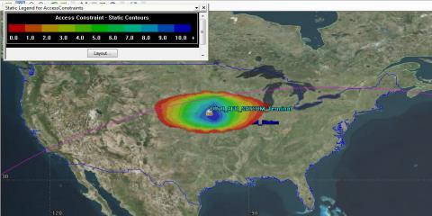
C/N Contours
- When finished, close the legend.
Grid Stats Over Time
The Grid Stats over Time report and graph summarize the minimum, maximum, and average of the Figure Of Merit's dynamic value over the entire grid as a function of time.
- Bring the Report & Graph Manager to the front.
- Generate a Grid Stats Over Time report.
- Note the optimum time for C/N?
- Save the Grid Stats Over Time report as a Quick Report.
- Uncheck the Coverage Definition object in the Object Browser.
- Close the report and the Report & Graph Manager.
Create an Area Target
You will use a custom built Area Target object, focusing in the area that had the highest C/N.
- Insert an Area Target object using the Insert Default method.
- Rename the Area Target object CommArea.
- Open CommArea's properties.
- On the Basic -Boundary page, make the following changes:
- Browse to the Basic - Centroid page.
- Make the following changes:
- Click OK.
| Option | Value |
|---|---|
| Area Type: | Ellipse |
| Semi-Major Axis: | 300 km |
| Semi-Minor Axis: | 200 km |
| Bearing: | 90 deg |
| Option | Value |
|---|---|
| Latitude: | 41 deg |
| Longitude: | -96 deg |
Communication Volumetric Analysis
The Spatial Analysis tool enables you to create calculations and conditions that depend on locations in 3D space which are, in turn, provided by user-definable volume grids. Combining spatial calculations and volume grids in volumetric objects allows you to report and graph calculations over time and across grid points, as well as visually depict volumes representing various values interpolated across grid points.
- In the Object Browser, right click on CommArea and select Analysis Workbench.
- When Analysis Workbench opens, click the Spatial Analysis tab.
- Click the Create new Volume Grid button.
- Ensure the Type is set to Cartographic and set the Name to CNVOL.
- Click the Set Grid Values button.
- Change both the Latitude and Longitude Number of Steps: to ten (10).
- Set the following values for Altitude:
| Option | Value |
|---|---|
| Minimum: | 1 km |
| Maximum: | 60 km |
| Number of Steps: | 20 |
- Click OK to close the Grid Values window.
- Click OK to close the Add Spatial Analysis Component window.
Create a Spatial Calculation
A Spatial Calculation is a calculation that depends on both time and location.
- Select DLRcvr in Object Tree.
- Click the Create new Spatial Calculation button.
- Ensure the Type is set to Scalar at Location.
- Set the Name to CN.
- Click the ellipsis button beside the Scalar option.
- Select the access object in the Object Tree (Facility-Offutt_AFB_SATCOM_Terminal-Receiver-DLRcvr-To-Satellite-CommSat-Sensor-TgtOffutt-Transmitter-DLXmtr).
- In the Scalar Calculation For: list, expand the CommLinkInformation data provider.
- Select C/N.
- Click OK to close the Select Reference Scalar Calculation window.
- Click OK to close the Add Spatial Analysis Component window.
Create a Time Component
The Time Tool is used to create components that produce instances or intervals of time.
- Click the Time tab in the Analysis Workbench tool.
- Change Filter by: to All Objects.
- Select the Scenario object (Comm_Constraints).
- Click the Create new Interval button.
- Set the Type to Fixed Interval and click OK.
- Set the name to MaxCN.
- Open the saved Grid Stats Over Time Quick Report.
- In the Maximum (dB) column, locate the time period that contained the highest reported values.
- Use the time period of that grouping to set the Start Time and Stop Time.
- Click OK.
- Close the Analysis Workbench.
- Leave the report open.
Add a Volumetric Object
The Volumetric object defines a 3-dimensional grid of points using various coordinate definitions, with respect to various reference coordinate systems from the Vector Geometry tool. It also defines the conditions and calculations that depend on locations in 3D space, and evaluates these conditions and calculations across grid points.
- Insert a Volumetric object using the Insert Default method.
- Open Volumetric object's properties.
- Click the Volume Grid: ellipses button.
- In the Object List, select CommArea.
- In the Volume Grids for: CommArea, select CNVOL.
- Click OK.
Add a Spatial Calculation
- Enable the Spatial Calculation option.
- Click the Spatial Calculation ellipsis button.
- In the Object List, select DLRcvr.
- In the Spatial Calculation for: DLRcvr list, elect CN.
- Click OK.
- Click Apply.
Set the Interval
- Select the Basic - Interval page.
- Click the Analysis Interval: ellipses button.
- In the Components for: Comm_Constraints list, select MaxCN.
- Click OK.
- Click Apply.
Calculate the Volumetric Object
Save your scenario.
- In the Object Browser, select the Volumetric object.
- At the top of STK extend the Volumetric menu.
- Click Compute. Be patient. This could take a few minutes.
Volumetric Graphics
- Select the 3D Graphics - Volume page.
- Enable the Spatial Calculation Levels option.
- Using the Grids Stats Over Time report note the highest values inside the time period used to create the Fixed Interval.
- Click the Insert Evenly Spaced Values... button.
- Enter zero (0) for Start Value and the highest value from the report for Stop Value.
- Leave the default Step Size.
- Click Create Values.
- Click OK.
View the Volumetric Object in 3D
Depending on the graphics capability of your computer, pressing the Start button in the Animation Tool Bar is not a good idea. As you cycle through the interval time, make sure you do it by using the Step Forward or Step in Reverse buttons.
- Set the Animation Time to the start value you used as the start value for the volumetric object.
- Change the Time Step: to 60.00 sec.
- Bring the 3D Graphics window to the front.
- Zoom To CommArea.
- Use the Step Forward button to slowly walk through the reported time period.
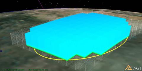
Volumetric Volume
Volumetric Values At Time
Values are computed at grid points at the specified time.
- In the Object Browser, right click on the Volumetric object.
- Select the Report & Graph manager.
- In the Styles list, select the Volumetric Values At Time report the click the Generate button.
- When the Report Time window opens, choose a date and time for the report.
- Click OK.
SAVE YOUR WORK!
 Visit AGI.com