STK Professional and Coverage.
The results of the tutorial may vary depending on the user settings and data enabled (online operations, terrain server, dynamic Earth data, etc.). It is acceptable to have different results.
Problem Statement
The Mount Saint Helens Worm Flows Route, from Marble Mountain Snow-Park, is the most direct route to the summit of Mount St. Helens during the winter season. Four ranger stations are used to perform visual observations of the trail. At times, only two stations are manned. You want to know which two observation posts, together, have the best percentage of visual coverage on the trail.
Solution
Build an STK scenario that analyzes the coverage of the four ranger stations used to monitor the Mount Saint Helens Worm Flows Route. Use STK Analyzer to perform a coverage analysis of the exercise area using all possible combinations of two of the four different station locations. Determine which combination of two stations provides the greatest percentage coverage along the hiking trail.
Create a New Scenario
Create a new scenario using the default analysis time period.
- Launch STK (
 ).
). - Click the Create a New Scenario (
 ) button.
 - Enter the following in the New Scenario Wizard:
- When you finish, click OK.
- When the scenario loads, click Save (
 ). A folder with the same name as your scenario is created for you in the location specified above.
 - Verify the scenario name and location and click Save.
- Close the Insert STK Objects tool (
 ).
).
| Option | Value |
|---|---|
| Name | Ranger Stations |
| Location | C:\Documents and Settings\<user>My Documents\STK 11 (x64) |
| Start | Accept Default Time |
| End | Accept Default Time |
Save Often!
Add Terrain and Imagery
If you have an Internet connection, you only need to add analytical terrain. Microsoft Bing Maps can be used for imagery. If you don't have an Internet connection, you can use imagery that is located in the STK install area.
- If you have previously created a *.pdtt file from the hoquiam-e.dem terrain data file during STK Comprehensive training or other advanced training, you can enable it for analysis in the Scenario's Properties . Basic - Terrain page.
- If you have not already created the *.pdtt file in a previous tutorial, we have provided one for you.
- When prompted Use Terrain for Analysis:
- If you are using the hoquiam-e.dem terrain data file for analysis, do not enable terrain for analysis.
- If you haven't loaded the hoquiam-e.dem terrain data file for analysis, enable terrain for analysis.
- If you do not have Microsoft Bing Maps (no Internet connection), you can load an imagery file (*.pdttx or *.jp2) to the globe in the 3D Graphics window.
- Select Use the Add Terrain/Imagery (
 ) option in the Globe Manager (
 ).
). - Browse to <STK install folder>\STKData\VO\Textures in the Path: drop down.
- Select St Helens.jp2 and click Open.
- Select Use the Add Terrain/Imagery (
- Right-click on StHelens_Training.pdtt in the Globe Manager and select Zoom To (
 ).
). - Right-click on StHelens_Training.pdtt in the Globe Manager and select Toggle Extents (
 ). Toggle Extents again to turn off the color overlay.
If you loaded the St Helens.jp2 file, you can zoom to it and toggle the extents from Globe Manager.
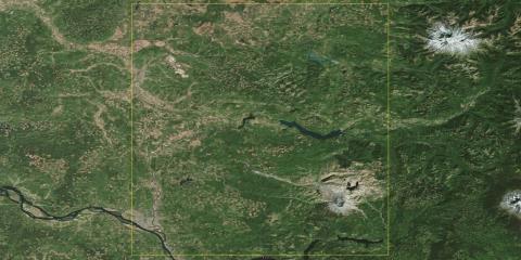
Terrain Region Display
Define Your Analysis Area
When using Globe Manager, the KML window is used to add Keyhole Markup Language (KML) files (.kml/.kmz) to a 3D Graphics window. Features specified in the KML files can be displayed or hidden and zoomed to using the KML window drop-down menu. As stated earlier, you are performing analysis along the Mt. Saint Helens Worm Flows Climbing Route. You would like to view the route as a model in the 3D Graphics window. You have a KMZ file that models the Mt. Saint Helens Worm Flows Climbing Route. You can use the STK Globe Manager to inlay the KML file for visualization in the 3D Graphics window. After you visualize the KMZ in STK, you can import it as an object to use for your analysis.
- In Globe Manager, click the KML tab.
- Click the Open KML Content icon (
 ).
). - Browse to the KML File located at <STK install folder>\Help\stktraining\KML.
- Select the file named MtStHelens.kmz and click Open.
- Click OK.
- Bring the 3D Graphics window to the front.
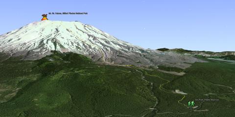
Mount Saint Helens Worm Flows Route
Build the Ranger Stations
There are four ranger stations along the hiking trail. The observation platforms are fifty feet high. You will build the first ranger station and then re-use it to create the other three ranger stations. By using Copy and Paste, all you will have to do is change the locations of the remaining three ranger stations.
- Click Insert on the Menu bar and select New... to open the Insert STK Objects tool ().
- Insert a Place (
 ) object using the Define Properties (
 ) method.
 - Set the following options on the Basic - Position page:
- On the Constraints - Basic page, make the following changes:
- Click OK to accept the changes and dismiss the Properties Browser.
- Right-click on the Place object in the Object Browser and Rename the place object "Station1".
- Select Station1 in the Object Browser and click the Copy (
 ) icon at the top of the Object Browser then click the Paste (
 ) icon three times.
 - One at a time, open the Properties of Station two through four and make the following property changes on their Basic - Position page:
| Option | Value |
|---|---|
| Latitude | 46.1488 deg |
| Longitude | -122.177 deg |
| Use terrain data | Enabled |
| Height Above Ground | 50 ft |
| Option | Value |
|---|---|
| Line of Sight | Disabled |
| Terrain Mask | Enabled |
| Latitude | Longitude |
|---|---|
| Station2: 46.1412 deg | -122.165 deg |
| Station3: 46.1638 deg | -122.184 deg |
| Station4: 46.1606 deg | -122.174 deg |
Station Coverage
You want to assess the coverage of any two of the four nodes along Mount Saint Helens Worm Flows Route. The Coverage Definition object defines a coverage area for analysis.
- Insert a Coverage Definition (
 ) object using the Insert Default Object tool. This will insert a new Figure of Merit and open its Properties Browser ().
Defining a Coverage Grid
Coverage analysis is based on the accessibility of assets (objects that provide coverage) and geographical areas. Define the location of a coverage grid.
- On the Basic - Grid page of the Coverage Definition () object's properties (), define the location of a coverage grid in the Grid Area of Interest field.
- On the Basic - Grid page, define the grid in the Grid Definition field:
- On the Basic - Grid page, define grid constraints using Grid Constraint Options.
| Option | Value |
|---|---|
| Type | Custom Boundary |
| Select Boundaries | Mount_Saint_Helens_Worm_Flows_Route |
| Option | Value |
|---|---|
| Point Granularity | Distance - 10 ft |
| Point Altitude | Altitude above Terrain - 0 km |
| Option | Value |
|---|---|
| Reference Constraint Class | Place |
| Use Object Instance | Enabled - Station1 |
Coverage Assets
Assets properties allow you to specify the STK objects used to provide coverage.
- On the Basic - Assets page, assign all four stations.
- Click Apply.
Coverage Interval
For this coverage scenario, you have static assets covering a static area. If you compute the coverage over the whole scenario time, that would be a waste of computations. None of the objects will change positions over time, so you can shorten the computation time.
- On the Basic - Interval page, click the drop down arrow and select Replace With Times.
- Change Stop to: + 1 sec.
Advanced Options
Advanced properties allow you to adjust the manner in which access information is stored and computed. Although it is not required, the possibility exists that after computing coverage, you might change the properties of an asset. Therefore, set up the Coverage Definition object to allow you to manually compute coverage.
- On the Basic - Advanced page, disable Automatically Recompute Accesses.
2D Graphics Display of the Coverage Grid
Later in the scenario, you will display color contours along the route. In order to better visualize the contour colors, remove the grid points along the route.
- On the 2D Graphics - Attributes page, in the Grid field, disable the Show Points option.
- Click OK to accept changes and dismiss the Properties Browser..
Compute Accesses Tool
The Compute Accesses tool allows you to compute accesses between the grid points and the assigned assets.
- Highlight the Coverage Definition () object in the Object Browser.
- Select CoverageDefinition in the Menu bar and select Compute Accesses.
Coverage Results
The Coverage Figure of Merit object enables you to analyze coverage in various directions over time, using several attitude-dependent figures of merit.
- In the Object Browser, select the Coverage Definition object.
- Insert a Figure of Merit (
 ) object using the Insert Default Object tool. This will insert a new Figure of Merit and open its Properties Browser ().
Measuring Number of Assets
Prior to running a trade study in Analyzer, determine how much of the route can be observed when utilizing all four stations. N Asset Coverage measures the number of assets available simultaneously during coverage.
Figure of Merit Reports
You want to determine the overall percentage of coverage along the route when at least one station is in use. The Percent Satisfied report presents the percentage of the total grid area and actual area where the static value of the Figure Of Merit meets the specified satisfaction criterion.
- Open the Report & Graph Manager (
 ).
). - Change Object Type to FigureOfMerit and select the Figure of Merit.
- Generate a Percent Satisfied report.
- Close the report and the Report & Graph Manager.
The percentage of coverage along the route when using all four stations. You'll compare this number to your analysis when using Analyzer.
Contours
You can specify how levels of coverage quality display in both the 2D and 3D Graphics windows. To accurately display contour levels for figures of merit in the 2D and 3D Graphics window, you should know the approximate range of values for the current Figure Of Merit. You have four stations being used in your coverage analysis. Based on your Percentage Satisfied report, you don't have 100% coverage. There are obvious gaps in the coverage. So, your contour range will be zero (o) through four (4).
- Return to the Figure of Merit () object's properties () and browse to the 2D Graphics - Animation page.
- Disable Show Animation Graphics.
- On the 2D Graphics- Static page, in Show Points As field, change Filled Area - % Translucency to ten (10).
- Enable Markers and leave the default marker.
- Steps three and four allow you to better visualize your contours along the route.
- In the Display Metric field, enable Show Contours.
- In the Level Attributes field, select the Remove All option.
- Make the following changes in the Levels field:
- Click the Add Levels option in the Level Attributes field.
- Enable the Color Ramp option and make the following changes to Color Method:
- Click the Legend... button.
- Click the Layout... button.
- Select the Show at Pixel Location in either the 2D Graphics Window.
- Click OK and then close the floating legend layout window. You should see a legend in the 2D Graphics Window.
| Option | Value |
|---|---|
| Level Adding | Start, Stop, Step |
| Start | 0 |
| Stop | 4 |
| Step | 1 |
| Option | Value |
|---|---|
| Start Color | Red |
| End Color | Blue |
You cannot view Line Target object contours in the 3D Graphics window.
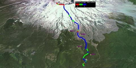
If you zoom into the route, you can see the color contours representing how many stations can simultaneously observe that portion of the route.
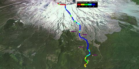
Color Contours
STK Analyzer
STK Analyzer automates STK trade studies and parametric analysis by blending the engineering analysis capabilities of Phoenix Integration, Inc.'s ModelCenter with AGI's STK software suite. Through its integration with the STK GUI and by using its own toolbars, Analyzer eliminates the need for scripts or programming. Now that you have determined the static coverage values for the route, run a trade study to determine which combination of nodes will result in the least degradation.
- Click Analysis on the menu bar, open the Analyzer menu and select Analyzer....
- In the scenario tree on the left, select the Coverage Definition () object.
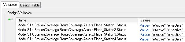
- In the STK Property Variables field, expand the Assets folder and then expand each station folder.
- Move, in order (1-4), all four Status variables to the Variables List on the right.
- Return to the STK variables tree and select the Figure of Merit () object.
- In the Data Provider Variables field, expand the Static Satisfaction folder.
- Move Percent Satisfied to the Variable List on the right.
You now have required inputs and outputs required for the trade study.
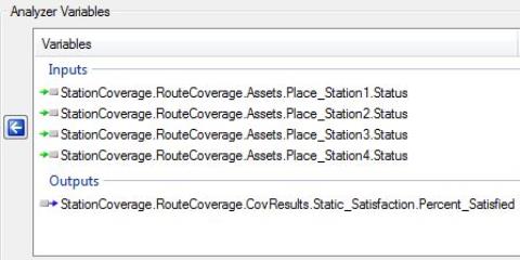
Analyzer Variables
Design of Experiments
The DOE (Design of Experiments) Tool is used to create and perform tables of runs for a Scenario. You can either use a classical design type, such as a Full Factorial design, or supply your own custom table of runs. You need to cover all possibilities of two stations being manned and two stations being unmanned. You are determining which two stations will provide the highest percentage of coverage.
- From the Component Tree on the left, drag and drop each Status, in order (1 through 4) to the Design Variables field.
- Return to the Component Tree and drag and drop Percent_Satisfied to the Responses field.
- Select the Design Table tab.

DOE Tool
Design Variables
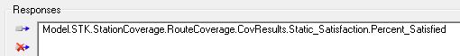
Responses
Design Table
The Design Table section contains a number of tools for editing design matrices. The user can directly edit values, add runs and delete runs. These edited designs can also be saved for later recall or imported from lists of comma separated values. If you look at the default table, there are multiple runs. Each Status column represents a station. You do not need to manually enter values into the table. You only need to delete each run that does not have a combination of two eInactive and two eActive cells.
- Remove all runs that do not have a combination of two eInactive and two eActive cells.
- Click Run... to run the analysis.
- Remember which two ranger stations resulted in the highest percentage of coverage, close down the Data Explorer, the DOE Tool, and Analyzer.
- Return to the 2D Graphics window.
When you have completed the design table, you should have a total of six runs (scenarios) that cover each possibility of two stations active and two stations inactive.
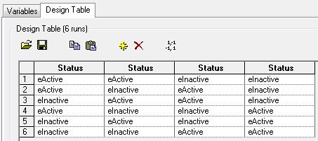
Completed Design Table
When the run is complete, look at the table. You can see which run has the highest percentage of coverage. Based on the following picture, you can see that when stations two and four (eActive) are manned, they present the highest percentage of visual observation along the trail. Therefore, on days that only allow for manning two ranger stations, stations two and four are the best choice.

Table
View Results In STK
Using the run that resulted in the highest percentage of coverage along the route, you can change the Coverage Definition object assets and the Figure of Merit contours to reflect and visualize the coverage along the route.
- Visualize the route in the 2D Graphics window to see the changes.
Active Stations
When finished, don't forget to save your work.
 Visit AGI.com