Problem Statement
Space Environment and Effects Tool (SEET) and STK Professional.
The Vehicle Temperature component estimates the mean temperature of a satellite due to direct solar and reflected Earth radiation, using simple thermal balancing equations. The nominal case is for a spherical satellite; optionally, this component can compute the temperature on a planar surface of specified geometry and orientation. As a DMSP satellite operator, determine the variation of the mean temperature of a satellite panel.
The results of the tutorial may vary depending on the user settings and data enabled (online operations, terrain server, dynamic Earth data, etc.). It is acceptable to have different results.
Break It Down
The following information should be determined before developing a Vehicle Temperature model scenario using STK:
- The vehicle shape is represented by a flat surface panel.
- The area and orientation of the panel of interest is 0.8 m2 normal to Earth.
- The emissivity, absorptivity and heat dissipation characteristics of the material(s) comprising the panel are 0.924, 0.248, and 010 respectively.
- Earth albedo should be set within the supported range that most closely approximate the conditions expected to be encountered during the mission.
Solution
Use STK and STK SEET to determine the variation of the mean temperature of a DMSP panel.
Create a Scenario
- Create a new scenario by using the New Scenario Wizard. You can also extend the File menu and select New...
- Rename the scenario SEET_VehicleTemperature.
- Set the analysis period to the following:
Option Value Analysis Start Time 1 Jul 201616:00:00.000 UTCG Analysis End Time 2 Jul 2016 16:00:00.000 UTCG
Add a Satellite
Add a satellite to the scenario that exercises the Vehicle Temperature model
- Insert a new satellite using the following method:
- Click the Insert button.
-
Set the following options in the Orbit Wizard.
Option Value Name Sat_VehicleTemp Type Orbit Designer Semi-major axis 7000 km Eccentricity 0.0 Inclination 110 degrees Argument of Perigee 0.0 RAAN 15 True Anomaly 0.0 - Click OK.
- Close the Satellite Database tool.
- Close the Insert STK Objects tool.
| Option | Value |
|---|---|
| Select an Object to be Inserted: |
 Satellite Satellite |
| Select a Method |
 Orbit Wizard Orbit Wizard |
Configure the Magnetic Field Model
Decide which field model(s) to use. The IGRF main-field with the Olson-Pfitzer external field gives the highest accuracy. Fast-IGRF is reasonably accurate alter-native to the IGRF (within 1%) which offers some improvement in speed. The centered-dipole model is a good choice when computational speed is a high priority. Analysis under about 15000 km altitude generally do not require the external field model.
Choose the IGRF update rate. The harmonic coefficients of the IGRF main-field change slowly with time and are maintained in tables having nodal values added every five years typically. Between these nodes, the coefficients are linearly interpolated. The “update rate” determines how frequently the IGRF model coefficients are re-interpolated from the table. The default of one (1) day should be fine for most circumstances, but increasing this value to up to 30 days for very long orbits can improve computational speed.
- Open the satellite's () properties (
 ).
). - Select the Basic - SEET Thermal page.
The properties related to the calculation of satellite temperature will be displayed on the Thermal Model page.
Configure the DMSP Satellite
- Set the Shape Model to Plate.
- Set the Cross-Sectional Area to 0.8 m2.
- Set the Normal Vector to Sat_VehicleTemp Earth. The normal vector identifies the orientation of the plate to Earth. For this tutorial, use the default value for albedo, which is near the center of the usual range of this value. If you'd like, you can tailor the scenario to more extreme conditions by modifying the Earth Environmental properties.
- Click OK.
Animate the Scenario
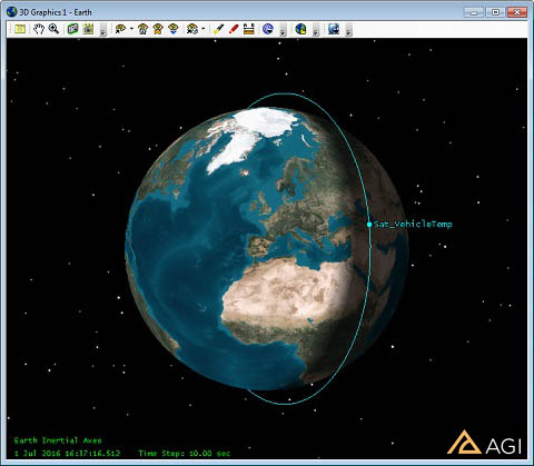
- Bring the 3D Graphics window to the front.
- Play (
 ) the scenario.
 - Reset (
 ) the scenario when finished.
 - Save (
 ) the scenario.
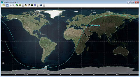
Notice that the satellite's orbital plane appears to maintain itself over the Earth's terminator, especially if viewed from the pole.
Create a Report of the Surface Temperature of the Satellite Panel
- Open the Report & Graph Manager (
 ).
). - Click the New Report (
 ) button.
 - Enter a name for the report like VehicleTemp.
- Expand (
 ) the SEET Vehicle Temperature Model Data Provider.
 - Move (
 ) the Definition field to the Report Contents field.
 - Click the New Section button.
- Double-click the SEET Vehicle Temperature Data Provider. This will move all of those contents to the second section of the report.
- Click OK.
- Generate the VehicleTemp report.
You will notice that the temperature varies slightly over time. Let's take a look at this in a graph.
Create a Vehicle Temperature Graph
- Click the New Graph Style (
 ) button.
 - Enter a name for the Graph like VehicleTemp.
- Expand () the SEET Vehicle Temperature Data Provider.
- Move () Temperature to the Y-Axis.
- Click OK.
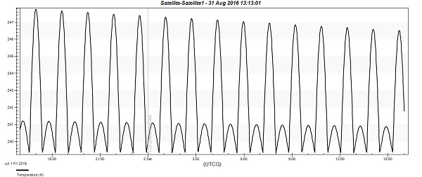
- Generate the VehicleTemp graph.
Results and Analysis
From the report and graph, one concludes that the mean panel temperature fluctuates by about eight degrees Celsius during the scenario considered. This rather constant temperature is not unexpected because the panel is not afforded an opportunity to escape solar heating by entering the shadow of the Earth, based on the report which indicates 100% percent solar intensity over many revolutions.
 Visit AGI.com