STK Professional, Analysis Workbench, Coverage, Communications, Radar, Aviator.
Before You Begin
This is an advanced tutorial that covers the new features in STK 11 and is designed to take approximately three (3) hours to complete. This tutorial assumes that the user has an understanding of STK Fundamentals.
Some of the sections in this tutorial require Internet ( ) for online operations. They are marked appropriately. If internet/online operations are blocked/disabled (
 ), there are additional steps for offline use. The status bar located at the bottom of STK displays the icons if you are online or offline. You can click on that icon to access the Help documentation and manage these settings depending on your network environment.
Several data files are provided for this scenario in the following directory: <STK Install Folder>\Help\stktraining\samples\SeaRangeResources
All data used in this tutorial was obtained from publicly available sources and is meant for training purposes only.
Problem Statement
In this tutorial, you will use STK to design a test plan at the Sea Range at Point Mugu, CA. This plan will be used to test the performance of several systems on a next generation, multi-role, unmanned aircraft vehicle (UAV). This tutorial is broken out into individual sections that help design this test plan using some of the new key features in STK 11. When you finish, you will be able to:
- Model the sea range in STK
- Model a mobile telemetry antenna using STK Terrain Server
- Model the airspace that has visibility to the telemetry antenna using Volumetric
- Model the UAV flight plan using Aviator
- Model the DDG ship-based radar tracking the UAV using Phased Array and Volumetric (Optional section)
- Model the satellite communications for the UAV using Phased Array and Volumetric
Solution
Use the new features in STK 11 to model and analyze the UAV systems at the Sea Range.
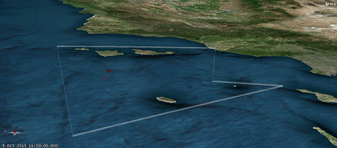
Model the Sea Range at Point Mugu
The Sea Range at Point Mugu, CA is the US Department of Defense’s largest and most extensively instrumented over-water range that offers realistic, open-ocean and littoral operation environments. This range will be used for the area of operations for this and all following scenarios.
The airspace for this exercise will be a subset of the overall airspace available at the Sea Range. The analysis will take place up to 40,000 feet.
Create a New Scenario
Create a new scenario using the default analysis start time and lasting 3 hours.
- Launch STK (
 ) (we recommend using the 64-bit version).
 - Create a New scenario (
 ) and name it STK11_SeaRange.
 - Use the default time period and change the Stoptime to +3 hours.
- Click OK to create the scenario.
- Save (
 ) the scenario.
Model the Available Airspace Boundary
Insert a new area target and define the properties.
- Bring the Insert STK Objects (
 ) tool to the front.
 - Insert and Area Target object (
 ) using the Define Properties (
 ) method.
 - Click the Add button to insert the following coordinates to create the area target boundary:
| Latitude | Longitude |
|---|---|
| 34.1 deg | -120.6 deg |
| 32.8 deg | -120 deg |
| 33.5 deg | -118.7 deg |
| 33.5 deg | -119.2 deg |
| 34.2 deg | -119.2 deg |
STK also allows you to create an area target boundary by using the 3D Object Editing tool and clicking where you'd like. You can also import KML or Shapefiles.
View the Airspace Boundary
Let's take a look at the boundary in 2D and 3D.
- Right-click on the Area Target object () in the Object Browser and select Rename.
- Rename the area target to Airspace.
- Right-click on Airspace and select Zoom To..
- Mouse around so you can see the region.
Clean Up the Graphics Windows
Let's take a moment to visually clean up the 2D and 3D Graphics windows.
- Open Airspace's () Properties ().
- Select the 2D Graphics - Attributes page.
- Set the following options:
- Select the 3D Graphics - Attributes page.
- Set the following options:
- Click OK to apply the changes to the area target and dismiss the Properties Browser.
| Option | Value |
|---|---|
| Color | White |
| Inherit from Scenario | Off |
| Show Label | Off |
| Show Centroid | Off |
| Option | Value |
|---|---|
| Show Boundary Wall | On |
| Upper Edge | WGS84 Ellipsoid (default) |
| Height from WGS84 | 1 km |
| Use Wall Translucency | On |
| Use Line Translucency | On |
Place DDG in the Center of the Airspace
Let's build the route of the DDG.
- Bring the Insert STK Objects () tool to the front.
- Insert a Ship object (
 ) using the Define Properties () method.
 - Set the Altitude Reference to MSL.
- Set the Route Calculation Method to Specify Time.
- Click the Insert Point button.
- Enter the following values:
- Click the Copy Point button.
- Change the second point time to the scenario end time.
- Click OK.
- Rename the Ship () object to DDG.
- Zoom To DDG ().
| Latitude | Longitude |
|---|---|
| 33.5 deg | -120 deg |
Fix the Ship's Position and Lighting
You may notice that the model is dark and below the surface of the Earth. We can fix that.
- Open STK11_SeaRange's () properties ().
- Select the 3D Graphics - Global Attributes page.
- Set the Surface At to Mean Sea Level.
- Click OK.
- Open the 3D Graphics window properties ().
- Select the Lighting page.
- Enable the Flashlight Show option and set the color to White.
- Set the Flashlight Level to 75.
- Select the Annotation page.
- Set the following values:
- Click OK.
- Save the scenario.
| Option | Value |
|---|---|
| Show Time Step | Off |
| Time Color | White |
| View Reference Frame | Off |
| Compass | On |
| Compass X and Y Position | 75 |
Model the Mobile Telemetry Antenna Using STK Terrain Server
In order to receive telemetry for this exercise, you will be using a mobile telemetry antenna on San Nicolas Island (SNI). SNI is a US Navy owned and operated island providing support for conducting test and training exercises. In order to receive telemetry, you must maintain line-of-sight with the aircraft throughout the entire mission. Additionally, you must take terrain into account since the island has mountainous terrain.
Add Terrain Using STK Terrain Server ()
- Open STK11_SeaRange's () properties ().
- Select the Basic - Terrain page.
- Ensure the Terrain Server option to Use terrain server for analysis is enabled.
- Enable the Analysis Operations for Line-Of-Sight Terrain Mask, Azimuth/Elevation Mask, and Coverage.
- Click OK.
- Open Globe Manager (
 ).
). - Ensure the World Terrain option is enabled
You can click the Edit Preferences... option to change from AGI's public terrain server to your private terrain server.
Add Terrain Without STK Terrain Server ()
If the STK Terrain Server is unavailable, follow the steps below to use the local files.
- Browse to the <STK install folder>/Help/stktraining/imagery using Windows Explorer.
- Drag and drop PtMugu_ChinaLake.pdtt onto the 3D Graphics window.
- Click Yes to use the terrain file for analysis.
- Open Globe Manager ().
- Right-click on PtMugu_ChinaLake.pdtt and select Properties ().
- Set the Altitude Scale to five (5) and view the 3D Graphics window to see the exaggerated terrain.
- Set the Altitude Scale back to one (1).
Insert a Facility and Compute the Az/El Mask
- Bring the Insert STK Objects () tool to the front.
- Insert a Facility object (
 ) using the Define Properties method.
 - On the Basic - Position page, make the following changes:
- On the Basic - AzElMask page, make the following changes:
-
Option Value Use Terrain Data Use Mask for Access Constraint On
| Option | Value |
|---|---|
| Latitude | 33.2798 |
| Longitude | -119.522 |
| Use terrain data | On |
Visualize the Terrain Mask
- Select the 2D Graphics - AzElMask page
- Enter the following options in the At Range section
- Click OK.
- Rename the Facility object to San_Nicolas.
- Zoom To San_Nicolas () and mouse around so you can see the AzElMask.
- Right-click on San_Nicolas () and select the Report & Graph Manager (
 ) option.
 - Generate an Azimuth-Elevation graph.
| Option | Value |
|---|---|
| Show | On |
| Number of Steps | 5 |
| Minimum Range | 0 km (default) |
| Maximum Range | 5 km |
| Color | White |
Move the Mobile Telemetry Antenna to Improve Line-of-Sight
Since we are on the shore of the island, we have poor line-of-sight due to the mountainous terrain of the island. Because you are using a Mobile Telemetry Antenna, you can move to a different location to improve your coverage.
- Select the Basic - Position page in the San_Nicolas' () properties().
- Set the following options to change your position:
- While looking at the value of Altitude: click Apply. You will notice the altitude update.
-
Bring the 3D Graphics window to the front and Zoom To San_Nicolas ().
-
Return to the Azimuth-Elevation graph and click the Refresh (
 ) button or hit F5.
-
When finished, close the graph and the Report & Graph Manager ().
-
Save () the scenario.
| Option | Value |
|---|---|
| Latitude | 33.2706 deg |
| Longitude | -119.521 deg |
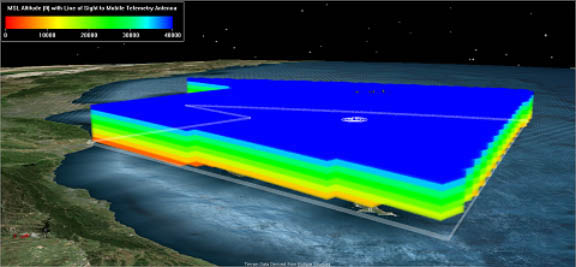
Model the Airspace that has Visibility to the Telemetry Antenna
Now that our mobile telemetry antenna is in place, we can use Volumetrics to analyze where we have visibility to our airspace. Volumetrics allows you to grid up volumes of space based on customized regions. In this case, we will set up a grid based on the area target, up to 40,000 ft at 5,000 ft intervals.
Save STK11_Volumetrics as a New Scenario
- Select STK11_SeaRange () in the Object Browser.
- Extend the File menu and select Save As.
- In the Save As pop up window, click the STK User option in the upper-left.
- Click the Create New Folder (
 ) button.
 - Name the new folder STK11_Volumetrics.
- Click Open.
- Change File Name to STK11_Volumetrics and click Save.
Define the Reference Grid Using the Spatial Analysis Tool
- Right-click on Airspace () and select Analysis Workbench.
- Select the Spatial Analysis tab.
- Click the New Volume Grid (
 ) button.
 - Set the Name to AirspaceVolume.
- Click the Set Grid Values... button.
- Set the Latitude and Longitude Number of Steps to 50.
- Set the following values for Altitude:
- Click OK to accept the Grid Values.
- Click OK to create the AirspaceVolume Grid.
| Option | Value |
|---|---|
| Minimum | 0 km (default) |
| Maximum | 40000 ft |
| Number of Steps | 8 |
Constrain Grid by Visibility
- Click the Create new Volume Grid () button.
- Click Select... to change the Type: to Constrained.
- Set the Name to AirspaceSanNicolasLOS.
- In the Reference Grid: field, click the ellipsis (
 ) button.
 - Select Airspace in the Objects field on the left.
- Select AirspaceVolume in the Volume Grids for Airspace field on the right.
- Click OK to close the Select Reference Volume Grid window.
- In the Spatial Condition: field, click the ellipsis () button.
- Select San_Nicolas in the Objects field on the left
- Select Visibility in the Spatial Conditions for San_Nicolas field.
- Click OK to close the Select Reference Spatial Condition window.
- Click OK to close the Add Spatial Analysis Component window.
Create the interval for analysis.
- Click the Time tab of the Analysis Workbench.
- Select the Scenario () object on the left.
- Click the Create new Interval (
 ) button.
 - In the Add Time Component window, make the following changes.
- Click OK to close the Edit Component Properties window.
- Close the Analysis Workbench.
| Option | Value |
|---|---|
| Type | Fixed Duration |
| Name | OneSec |
| Stop Offset | 1 sec |
Create the Volumetric Object
- Bring the Insert STK Objects () tool to the front.
- Insert a Volumetric object (
 ) using the Define Properties () method.
 - Click the ellipsis (
 ) button to change the Volume Grid.
 - Select Airspace on the left and select AirspaceSanNicolasLOS gird on the right.
- Click OK.
- Click Apply.
- Browse to the Basic – Interval Page.
- Click the ellipsis () button to change the Analysis Interval.
- Select the OneSec interval created in the previous section, then click OK.
- Browse to the 3D Graphics – Grid page.
- Set the grid point Size to 2.
- Disable the Show grid lines checkbox.
- Click Apply.
Compute the Volumetric Object
- Right-click on Volumetric1 () and extend the Volumetric menu.
- Click Compute.
- Right-click on Volumetric1 () and select Report & Graph Manager ().
- Expand (
 ) the Installed Styles directory and generate the Satisfaction Volume report.
Define a Spatial Calculation Based on Altitude
- Open Volumetric1's () Properties ().
- Select the Basic - Definition page.
- Enable the Spatial Calculation checkbox.
- Click the ellipsis () button.
- Select the Airspace on the left and select Altitude on the right.
- Click OK.
- Click Apply.
Define the Graphics of the Volume
- In the Volumetric1's () Properties (), select the 3D Graphics - Volume page.
- Select the Spatial Calculation Levels option at the top.
- Click Insert Evenly Spaced Values... to set the contour levels to the following values:
- Click the Create Values button.
- Select the 3D Graphics - Legends page.
- Enable the Show Legend.
- Change the title of the legend to "Altitude (ft)"
- Set the Color Square Width (pixels) to 100.
- Click Apply.
| Option | Value |
|---|---|
| Start | 0 |
| Stop | 40000 |
| Step | 5000 |
Disable Volumetric's Graphics
- Save () the scenario.
- Disable the Volumetric1 () object to disable the graphics.
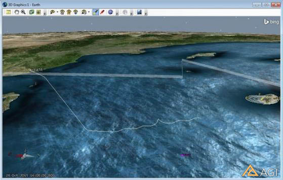
Model the X-47B UAV route using Aviator
You analyzed the Sea Range airspace and determined the acceptable flight volumes. Now you’ll model an aircraft route using that information. Additionally, the aircraft will fly to the DDG and perform a variety of maneuvers. You will analyze the stealth performance against the DDG’s radar.
Save STK_Aviator as a New Scenario
- Extend the File menu.
- Click the Save As option.
- In the Save As pop up window, click STK User.
- Click the Create New Folder button.
- Name the new folder STK11_Aviator.
- Click Open.
- Change File Name to STK11_Aviator and click Save.
Import ARINC 424 Data
- Extend the STK Utilities menu.
- Select Aviator Catalog Manager.
- Select Runway - AIRINC424runways.
- Click the ellipsis () button and browse to the Master Data File (<STK install folder>/Help/stktraining/samples).
- Open FAANFD18.
- Click Save.
- Close the Aviator Catalog Manager.
Insert the X-47B Aircraft Using the Standard Object Database ()
- Bring the Insert STK Objects () tool to the front.
- Insert an Aircraft object (
 ) using the From Standard Object Database (
 ) method.
 - Search for "x-47" in the Name field, then hit Enter.
- Select X-47B in the results and click Insert.
- Close the Standard Object Database.
- Open X-47B's () Properties ().
Insert the X-47B Aircraft using Local Files ()
Note: You can skip this section if you've already inserted the X-47B from the standard object database using the online steps above.
- Extend the STK Utilities menu and select the Aviator Catalog Manager.
- Expand (
 ) the Aircraft option.
 - Right-click on User Aircraft Models and select Import.
- Browse to <STK install folder>/Help/stktraining/samples/X-47B and open the X-47B_PerformanceModel.eximpkg file.
- Click Import.
- Click Save then close the Aviator Catalog Manager.
- Bring the Insert STK Objects () tool to the front.
- Insert and Aircraft object () using the Define Properties () method.
- Change the Propagator to Aviator.
- Click the Select Aircraft (
 ) button and change the type to X-47B.
 - Select the 3D Graphics - Model page.
- Change the model file (<STK install folder>/Help/stktraining/samples/X-47B/X47B_UCAV_Cert_v48.mdl).
Takeoff from Point Mugu Using ARINC 424 Data
-
In the X-47B Basic - Route properties page, click the Insert Procedure After button (
 )
) - Select Runway from Catalog.
- Enter "mugu" in the Filter: search field, then hit Enter
- Select Point Mugu NAS (Naval Base VEN 03 21).
- Click Next.
- Select Takeoff.
- Select the option Use runway heading 212 Mag 224 True.
- Click Finish.
- Click Apply.
- If a message pops up with a flight path warning, click the Set Globe Reference to MSL button.
Fly to DDG
The test plan calls for the aircraft to fly ten (10) nm from the DDG, then perform a series of weave and barrel roll procedures to test the observability of the UAV.
- Right-click on the Takeoff procedure and select Insert Procedure After.
- Select STK Object Waypoint and link to DDG.
- Set the Offset Mode to Bearing/Range (relative to North).
- Set the Range to ten (10) nm.
- Click Next.
- Select Enroute and set the Altitude to 15000 ft MSL. You may have to disable "Use Aircraft Default Cruise Altitude" first.
- Set the name to Fly 10 nm from DDG.
- Set the Nav Mode to Arrive on Course.
- Set the Arrive on Course option to 180 deg (True).
- Click Finish.
- Click Apply.
- Save () your scenario.
Perform Maneuvers
The test plan calls for a series of maneuvers designed to test the stealth performance of the UAV against the DDG’s radar. Aviator allows you to define a variety of maneuvers.
- Right-Click on the Fly 10 nm from DDG procedure, then select Insert Procedure After.
- Select the End of Previous Procedure option and click Next.
- Select Basic Maneuver, then set the Name to Straight 2 nm.
- Ensure the default Straight Ahead Strategy is selected, and enable the Downrange stop condition.
- Set the Downrange stop condition to two (2) nm.
- Click Finish.
- Click Apply.
The “Help Me Choose…” button gives a brief description of each of the maneuver strategies. Click the Help to learn more.
Add the Weave Procedure
- Right-click on the Straight 2 nm procedure and select Insert Procedure After.
- Select the End of Previous Procedure option and click Next.
- Select the Basic Maneuver option and set the Name to Weave Twice.
- Set the Strategy to Weave and set the Max Number of Cycles to two (2).
- Click Finish twice.
- Right-click on the Weave Twice procedure and select Insert Procedure After.
- Select the End of Previous Procedure option and click Next.
- Select Basic Maneuver and set the Name to Barrel Roll.
- Set the Strategy option to Barrel Roll and click Finish twice.
- Right-click on the Barrel Roll procedure and select Insert Procedure After.
- Select the End of Previous Procedure option and click Next.
- Select the Basic Maneuver option and set the Name to Weave Twice Again.
- Set the Strategy to Weave and set the Max Number of Cycles option to two (2).
- Click Finish twice.
- Click Apply, then bring the 3D Graphics window to the front and view your flight route.
Add the Turn Around Procedure
- Right-click on the Weave Twice Again procedure and select Insert Procedure After.
- Select the End of Previous Procedure option and click Next.
- Select the Basic Maneuver option and set the Name to Turn left 270 deg.
- Set the Strategy option to Simple Turn and set the Relative Turn Angle option to -270 deg.
- Click Finish twice.
- Right-click on the Turn left 270 deg procedure and select Insert Procedure After.
- Select the End of Previous Procedure option and click Next.
- Select the Basic Maneuver option and set the Name to Turn right 90 deg.
- Set the Strategy option to Simple Turn and set the Relative Turn Angle to 90 deg.
- Click Finish twice.
- Click Apply.
- Save () your scenario.
Repeat Weave and Barrel Roll Maneuvers
Your test calls for the aircraft to fly by the ship twice. Now that you have turned around, you will use the same procedures listed above. However, rather than recreating all the steps, you can use a super procedure, which is a collection of individual procedures to repeat the series of weave and barrel roll procedures.
- Left-click and hold shift to multi-select the following procedures:
- Weave Twice
- Barrel Roll
- Weave Twice Again
- Right-click and select Copy, Paste, Edit > Copy Procedures.
- Right-click on the Turn Right 90 deg procedure and select Insert Procedure After.
- Select Super Procedure and set the name to Repeat Maneuvers.
- Click Next.
- Click the Load Procedures from Clipboard button and notice the 3 procedures are added.
- Click Finish.
- Click Apply.
- Save () your Scenario.
This will copy them to your Windows clipboard. Also note that the selected procedures are highlighted in the graph below.
Land back at Pt Mugu
- Right-click on the Repeat Maneuvers procedure and select Insert Procedure After.
- Select the Runway from Catalog option.
- In the Filter, type “mugu” then hit enter.
- Select the POINT MUGU NAS (NAVAL BASE VEN 03 21) option.
- Click Next.
- Select Landing.
- Set the Runway Altitude Offset to five (5) ft.
- Enable the Use Terrain for Runway Altitude option.
- Click Finish.
- Click Apply.
Ensure You Have Enough Fuel Accounting for Wind
- Right-click in the profile graph area below the procedures and select Profile Options / Properties.
- Enable the Secondary Y Axis option, select Fuel State, then click OK.
- Zoom in on the graph by dragging a box around the fuel state line near the end of the route.
- Hover your mouse to note the value. This does not take wind into account.
- Right-click in the graph and select Undo Zoom.
- Right-click on the Landing procedure, and select Profile data at Final State.
- Scroll through the list and note the value of Fuel State.
Enable Constant Wind ()
- Click the Wind (
 ) button to enable wind.
 - Set the Wind Speed to 50 nm/hr.
- In the atmosphere section, click the “Non Standard Surface Conditions” checkbox.
- Change the units (
 ) for the “Sea Level Temperature”, then set to 90 degF.
 - Click OK.
- Right-click on the Landing procedure and select Profile data at Final State.
- Scroll through the list and note the value of fuel state.
View the Impacts of Wind
- Right-click in the profile graph area below the procedures and select Profile Options / Properties.
- Set the Secondary Y Axis option to Course Crosswind and click OK.
- Right-click in the graph on one of the peaks and select Set Animation Time.
- Select the 3D Graphics – Vector page and click Add.
- Select the Aviator Wind vectorthen click OK.
- Enable the Show Magnitude checkbox.
- Set the Component Size Scale option to 1.0.
- Select the Axes tab, and enable the Body and VVLH(CBF) Axes options.
- Zoom To X-47B () and mouse around in the 3D Graphics window.
The Body axes is offset from the VVLH(CBF) Axes. This is referred to as a “crab angle,” which is the amount of correction an aircraft must be turned into the wind in order to maintain the desired course.
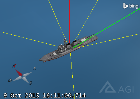
View the Aircraft Route
- Right-click on the Straight 2nm procedure and select Set animation time.
- Decrease (
 ) your time step to .5 sec.
 - Zoom To X-47B ().
- Play (
 ) to animate the scenario and watch your aircraft perform the maneuvers.
 - Pause (
 ) the animation.
 - In the timeline view, click the Add Time Components (
 ) button to add a new timeline component.
 - Select X-47B () on the left, and MissionProcedureIntervals on the right and click OK.
- Zoom in on the DDG (), then mouse around manually zoom out so you can see the aircraft route.
- Use the timeline view scroll bar to scroll through the entire mission.
- Save () the scenario.

(Optional) Enable dynamic wind from NOAA ADDS Service ()
- In the X-47B properties Basic - Route page, Click () to enable wind.
- Change the Model type to NOAA ADDS Service.
- Click the Manage Data… option.
- Click the Add Current Forecast button.
Note: This will pull data for the next 24 hour from today's date. If your scenario takes place in the past, this data will be unavailable.
- Click OK to accept and dismiss the ADDS Messages properties.
- In the atmosphere section, click the “Non Standard Surface Conditions” button.
- Change the units () for the “Sea Level Temperature”, then set to 90 degF.
- Click OK.
- Right-click on the Landing procedure and select Profile data at Final State.
- Scroll through the list and note the value of fuel state.
You can set up your own weather service by clicking the “Server Options” button. You can also export wind data for offline use or when saving your scenario with a date in the past.
- In the X-47B properties Basic - Route page, Click () to return to the wind settings.
- Change the Model Type to Constant Bearing/Speed.
- Set the Wind Speed to 50 nm/hr.
- Click OK.
- Save () the scenario.
Track the UAV using the DDG Phased Array Radar (Optional)
The X-47B route is built. Now you will model the phased array radar on the DDG, and then calculate the probability of detecting the X-47B. Although you won’t be modeling the full phased array radar on board the DDG, you would like to model some of the key parameters to get an understanding of the overall probability of detection.
Note: This section is optional. You may skip to the next section and still complete the tutorial.
Save STK11_Phased_Array_Radar as a New Scenario
- Extend the File menu.
- Click the Save As option.
- In the Save As pop up window, click STK User.
- Click the Create New Folder button.
- Name the new folder STK11_Phased_Array_Radar.
- Click Open.
- Change File Name to Phased_Array_Radar and click Save.
Model the Phased Array Radar
- Bring the Insert STK Objects () tool to the front.
- Insert and Radar object (
 ) using the Define Properties () method.
 - Attach the Radar to DDG ().
- Leave the type set to Monostatic.
The Bistatic Radar type allows you to model a different transmitter and receiver antennas for the Radar if necessary.
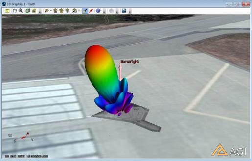
Model the Phased Array Antenna
- Select the Antenna tab.
- Set the Type from Parabolic to Phased Array.
- In the Element Configuration tab, set the number of X and Y elements to nine (9).
- In the Beam Direction Provider tab, enable the Beam Steering option.
- Double-click X-47B () as the beam target.
You can also steer the phased array beam based on the access object, an external data file, or a script.
The phased array antenna supports multiple beam targets.
Model the Transmitter
- Click the Transmitter tab.
- Set the Power to 60 dBW.
- Click Apply.
- Rename the Radar to DDG_PA_Radar.
Visualize the Phased Array Radar
- In the 3D Graphics – Attributes page, select Show Volume.
- Set the following options:
| Option | Value |
|---|---|
| Show as wireframe | On |
| Gain Scale (per dB) | .005 km |
| Gain Offset | 10 dB |
| Set azimuth and elevation resolution together option | On |
| Resolution | 3 deg |
Add a Vector
- Select the 3D Graphics – Vector page.
- Click the Add button.
- Select DDG on the left, then click the vector button to create a new vector.
- Set the Name to DDG_To_X-47B.
- Click the ellipsis () button to change the Origin Point.
- Select DDG on the left and Center on the right and click OK.
- Click the ellipsis () button to change the Destination Point.
- Select X-47B on the left and Center on the right, then click OK.
- Click OK.
- Select the DDG_To_X-47B vector and click OK.
- Enable the Show Magnitude option and set the units to nm.
- Zoom To DDG ().
- Animate () to watch the beam follow the displacement vector.
Import an External Radar Cross Section File
- Right-click on X-47B () and select properties ().
- Select the RF – Radar Cross Section page.
- Disable the Inherit checkboxto ignore scenario level settings.
- Set the Compute Type drop-down to External File.
- Click the ellipsis () button to browse to <STK install folder>/Help/stktraining/samples/SeaRangeResources/X-47B and open X-47B_Notional_Sample.rcs.
- Click Apply.
- Select the 2D Graphics – Radar Cross Section page.
- Enable the Show option.
- In the Level Adding section, set the following values.
- Click the Add Level button.
- Enter the following options:
- Click Apply.
- Select to the 3D Graphics – Radar Cross Section page.
- Zoom To X-47B () to view the RCS pattern.
This is a notional data file meant for training purposes.
| Option | Value |
|---|---|
| Start | 0 |
| Stop | -20 |
| Step | -5 |
| Option | Value |
|---|---|
|
Set theta and rho resolution together |
On |
| Resolution | 1 deg |
This will display the RCS (dBSm) relative to the max RCS.
| Option | Value |
|---|---|
| Show Lines | On |
|
Show Volume |
On |
| Scaled (per dBsm) | 1 m |
|
Set theta and rho resolution together |
On |
| Resolution | 1 deg |
Compute Probability of Detection of the UAV
- Right-click on DDG_PA_Radar () and select Access (
 ).
). - Select X-47B (), then click the Compute button.
- Click the Access… button to determine the intervals you have line of sight to the UAV.
- Click the AER… button to generate a time-history Graph of Azimuth, Elevation, Range.
- Click the Report & Graph Manager… button to bring up additional reports and graphs.
- In the Installed Styles, scroll down and double click to generate a Radar SearchTrack SNR graph.
- Right-click on the max SNR and select Set Animation Time.
- Close the graph and close the Access tool.
The max SNR occurs when the UAV is closest to the DDG and banking.

Analyze the Entire Range Airspace for Radar
You would like to ensure that the RF energy used for tracking the X-47B is maintained within your airspace and won’t impact additional aircraft outside the airspace. Since the radar will only be tracking during the maneuvers, use that as your analysis interval.
Create the volumetric object
- Bring the Insert STK Objects () tool to the front.
- Insert and Volumetric object () using the Define Properties () method.
- Click the ellipsis () button to browse to change the Volume Grid.
- Select Airspace on the left, and select AirspaceVolume on the right.
- Click OK.
- Click Apply.
- Select the 3D Graphics – Grid page, and set the following values:
- Click OK.
- Rename this Volumetric object to Vol_SNR
| Option | Value |
|---|---|
| Grid Point Size | 2 |
| Show Grid Lines | Off |
Create the volumetric grid template object
In order to evaluate the SNR across the volumetric grid, you can define a scalar calculation to a grid template object, and have that grid template object move to all the grid point locations defined in the volumetric object. Furthermore, you will need to compute access to that grid point template object so that the scalar calculation for SNR will exist.
- Bring the Insert STK Objects () tool to the front.
- Insert an aircraftobject () using the Define Properties () method.
- Set the Route Calculation Method to Specify Time.
- Click the Insert Point button on the right.
- Click the Insert Point button on the right again.
- Change the 2nd point Time to 19:01:00.
- Select the RF – Radar Cross Section page, then disable the Inherit option.
- Set the Constant RCS Value to 3dBsm.
Because this is a regional analysis for other aircraft, the actual aspect dependent rcs value of the “other” aircraft is unknown, so a constant RCS is more suitable than an aspect dependent RCS.
Compute Access
- Click OK.
- Rename the new Aircraft1 object to Vol_Grid_Template.
- Disable the Vol_Grid_Template graphics checkbox in the Object Browser.
- Right-Click on the DDG Radar (), and select Access ().
- Select Vol_Grid_Template and click Compute.
- Close the Access tool.
Create a Spatial Calculation for SNR based on Vol_Grid_Template
Now that you have computed access from the DDG radar to the Vol_Grid_Template, Analysis workbench has automatically created scalar calculations for all the available radar calculations, including SNR. You now need to create a spatial calculation that will move the Vol_Grid_Template to each location in the volumetric grid and evaluate the SNR at that location.
- Right-click on Vol_Grid_Template in the object browser and select Analysis Workbench.
- Select the Spatial Analysis tab.
- Click the new Spatial Calculation (
 ) button to create a new spatial calculation.
 - Ensure that the Type is set to Scalar At Location.
- Set the name to SNR.
- Click the ellipsis () button to change the Scalar.
- Expand the size of the current window so you can read all of the options.
- Select the access calculation from the DDG_PA_Radar to the Vol_Grid_Template on the left.
- On the right, select RadarSearchTrack > PrimaryPolarization > SNR1, then click OK.
- Click OK, then close Analysis Workbench.
- Save the scenario.
Update the Volumetric Object to Use the SNR Spatial Calculation
Now that you have the SNR spatial calculation, you will configure the Volumetric object to use that spatial calculation, compute the data, and configure the graphics.
- Open Vol_SNR's () Properties ().
- Enable the Spatial Calculation option.
- click the ellipsis () button.
- Select Vol_Grid_Template on the left and select SNR on the right.
- Then click OK.
- Click Apply.
- Right-click on Vol_SNR and select Volumetric > Compute.
This may take a while to compute. STK is performing detailed radar calculations.
Configure the Graphics of the Volume
- Select the 3D Graphics – Volume page and select the Spatial Calculation Levels option.
- Enable the Show Boundary Levels option.
- Disable the Show Fill Levels option.
- Click Insert Evenly Spaced Values... button to set the contour levels to the following values:
- Click the Create Values button.
- Disable the Immediately update graphics option.
- Set the Translucency for each level to 44%.
- Click Apply.
- Select the 3D Graphics – Legends page.
- Select the Boundary Legend tab.
- Enable the Show Legend option.
- Set the title to SNR (dB).
- Enter the following values:
- Click Apply.
- Zoom To DDG () then zoom out so you can see the whole airspace.
- Save () your scenario.
The min and max values of the spatial calculation in the upper-right.
| Option | Value |
|---|---|
| Start | -40 |
| Stop | 20 |
| Step | 10 |
| Option | Value |
|---|---|
| Number of Decimal Digits | 0 |
| Color Square Width (pixels) | 50 |

To animate your scenario, Volumetric sill needs to recompute the data at every time step. In order to compute all of the data beforehand to animate smoothly, adjust the Volumetric - Interval to use the "At times at step size" option, and set as desired.
Remove RCS, Volume Graphics and Vectors
- Open X-47B’s () properties ().
- Select the 2D Graphics – Radar Cross Section page.
- Disable the Show option.
- Select the 3D Graphics – Radar Cross Section page.
- In the Contour Graphics field, disable the Show Lines.
- In the Volume Graphics field, disable the Show Volume.
- Select the 3D Graphics – Vector page.
- Disable Aviator_Wind Vector Show.
- Select the Axes tab.
- Disable Show for both Body Axes and VVLH(CBF) Axes.
- Click OK.
Model the satellite communications for the UAV using Phased Array and Volumetric
You need to evaluate the performance of a phased array antenna on the X-47B to ensure adequate communications with a constellation of Low Earth Orbiting satellites. Additionally, you will need to evaluate the additional RF energy towards other communications satellites in Medium Earth Orbit and Geostationary Earth Orbit to ensure there are no interference impacts.
Save STK11_Phased_Array_SATCOM as a New Scenario
- Extend the File menu.
- Click the Save As option.
- In the Save As pop up window, click STK User.
- Click the Create New Folder button.
- Name the new folder STK11_Phased_Array_SATCOM.
- Click Open.
- Change File Name to Phased_Array_SATCOM and click Save.
Model the Template Satellite for the Constellation
You will be using a walker constellation to model the Low Earth Orbiting communication satellites. Each satellite will have a hemispherical nadir pointing antenna. In order to define the walker constellation, you first need to create a template satellite to define the general orbital parameters.
- Bring the Insert STK Objects () tool to the front.
- Insert and Satellite object (
 ) using the Orbit Wizard (
 ) method.
 - Set the following options:
- Click OK.
| Option | Value |
|---|---|
| Type | Repeating Sun Sync |
| Name | LEO_Comm_Sat |
| Approximate Altitude: | 800 km |
| Color | White |
Model the receiver
- Bring the Insert STK Objects () tool to the front.
- Insert a Receiver object (
 ) using the Define Properties () method.
 - Attach the Receiver to the LEO_Comm_Sat ().
- Set the Type to Complex Receiver Model.
- Click the Antenna tab and change the Type to Hemispherical.
- Click Apply.
- Select the 3D Graphics – Attributes page and enable the Show Volume option.
- Click OK.
- Rename the Receiver object SATCOM_Rx.
- Zoom To LEO_Comm_Sat ().
- Click (
 ) to change the view to home view and view the orbit of the satellite in the 3D Graphics window.
 - Play () to animate or scroll through the scenario to watch the satellite orbit the Earth.
Model the Walker Constellation Based on the Template Satellite
Now that you have your template satellite, you would like to create a constellation with those orbital characteristics that provide global coverage. You would like to design a constellation that has at least one satellite in view of the aircraft at all times.
- Right-click on LEO_Comm_Sat () in the Object Browser and extend the Satellite menu to select Walker, then set the following values:
- Click the Create Walker button.
- Click Close once the satellites have all been created.
| Option | Value |
|---|---|
| Type | Custom |
| Number of Planes | 10 |
| Number of Sats Per Plane | 10 |
| True Anomaly Phasing | 60 deg |
| RAAN Increment | 18 deg |
| Color by Plane | Off |
| Create Constellation | On |
| Name of Constellation | LEO_Comm_Sats |

Model the Phased Array Transmitter On-Board the X-47B
- Bring the Insert STK Objects () tool to the front.
- Insert and Transmitter object (
 ) using the Define Properties () method.
 - Attach the Transmitter to the X-47B ().
- Set the following options:
- Click the Antenna tab.
- Set the following options:
- Select the Beam Direction Provider tab.
- Enable the Beam Steering checkbox.
- Enable the Satellite Filter option.
- Move (
 ) all of the satellites to the beam target list.
 - Click Apply.
- Select the Orientation tab.
- Set the Elevation to -90 deg.
- Click Apply.
- Select the Constraints - Basic page, and set the Max Range to 2000 km.
- Click Apply
| Option | Value |
|---|---|
| Type | Complex Transmitter |
| Power | 40 dBW |
| Option | Value |
|---|---|
| Type | Phased Array |
| Element Configuration | Set X and Y to 9 |
Configure the Graphics of the Antenna Pattern
- Select the 3D Graphics - Attributes page.
- Set the following options:
- Select the 3D Graphics - Vector page.
- Enable the Boresight Vector option.
- Click OK.
- Rename the transmitter X47_Tx.
- Reset the animation time, and Zoom To X-47B.
- Save the scenario.
| Option | Value |
|---|---|
| Show Volume | On |
| Gain Scale (per dB) | .0005 km |
| Gain Offset | 10 dB |
| Set azimuth and elevation resolution together | On |
| Resolution | 2 deg |
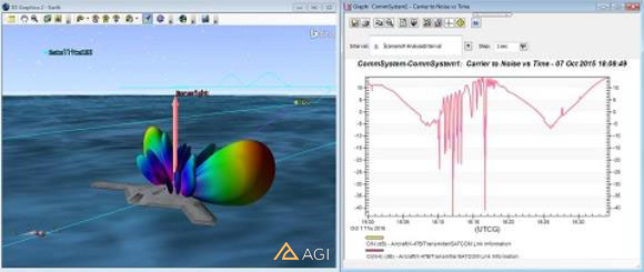
Plot C/N Along the Route
In order to compute the Carrier to Noise (C/N) ratio from the X-47B transmitter to the group of LEO SATCOM receivers, you will need to group these objects and use a Comm System object to compute the data.
- Bring the Insert STK Objects () tool to the front.
- Insert and Constellation object (
 ) using the Define Properties () method.
 - Assign the Transmitter (X47_Tx) () to the Constellation ().
- Click OK.
- Rename the Constellation, SATCOM_Tx.
- Bring the Insert STK Objects () tool to the front.
- Insert and Constellation object () using the Define Properties () method.
- Enable the Receiver Filter
- Movethe Receivers () to the Constellation ().
- Click OK.
- Rename the Constellation, SATCOM_Rx.
Build the Comm System
- Bring the Insert STK Objects () tool to the front.
- Insert a Comm System object (
 ) using the Define Properties () method.
 - Select the Basic - Transmit page and double-click the SATCOM_Tx constellation.
- Select the Basic - Receiver page and double-click the SATCOM_Rx constellation.
- Select the Link Definition page.
- Set the Constraining Constellations to Transmit.
- Click OK to apply these settings and close the Comm System properties.
If you do not see the Comm System object, click the Edit Preferences... button to add it to the Insert STK Objects panel.
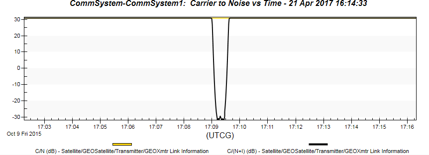
Compute the CommSystem and Plot the C/N
- Right-click on the CommSystem () object in the Object Browser.
- Extend the CommSystem menu and select Compute Data.
- Right-click on the Comm System () object in the Object Browser and launch the Report & Graph Manager ().
- Generate the Carrier to Noise vs Time graph.
- Set the Step size to 1 sec, then refresh the graph.
- Close the graph and the Report and Graph manager.
Analyze the RF output throughout MEO
You would like to ensure that the RF energy used for communications doesn’t interfere with other satellite communications beyond MEO to GEO. In order to evaluate the CN across the MEO, you can define a scalar calculation to a grid template object, and have that grid template object move to all the grid point locations defined in the volumetric object.
Create the Volumetric Object
- Bring the Insert STK Objects () tool to the front.
- Insert and Volumetric object () using the Define Properties () method.
- Click the ellipsis () button to browse to change the Volume Grid.
- Click the New Volumetric Grid () option.
- In the Add Volumetric Component window, set the following options:
- Click the Set Grid Values button and set the following Longitude options:
- Set the following Altitude changes:
- Click OK.
- Select MEO_West and click OK.
- Click Apply.
| Option | Value |
|---|---|
| Type | Cartographic |
| Name | MEO_West |
| Parent | CentralBody/Earth (default) |
| Option | Value |
|---|---|
| Minimum | -180 deg |
| Maximum | 0 deg |
| Number of Steps | 10 |
| Option | Value |
|---|---|
| Minimum | 2000 km |
| Maximum | 36000 km |
| Number of Steps | 5 |
Change the View
- Select the 3D Graphics - Grid page.
- Set the following values:
- Click OK.
- Rename the Volumetric object to Vol_CN.
- View the Volumetric Object in the 3D Graphics window by clicking the home view icon and mousing around.
| Option | Value |
|---|---|
| Grid Point Size | 2 |
| Show Grid Lines | Off |
Define the Volumetric Grid Template Object
We can use our template satellite that we used to define our walker constellation as our volumetric grid template object. In order to do this, you will need to compute access to that grid point template object so that the scalar calculation for CN will exist.
- Right-click on X47_Tx () in the Object Browser.
- Click Access ().
- Select LEO_Comm_Sat > SATCOM_Rx ().
- Click Compute.
- Close the Access tool.
Create a Spatial Calculation for SNR Based on Vol Grid Template
Now that you have computed access from the X-47B to the Leo_Comm_Sat template satellite, Analysis workbench has automatically created scalar calculations for all the available communications calculations, including CN. You now need to create a spatial calculation that will move the template object to each location in the volumetric grid and compute the CN at that location.
- Right-click on LEO_Comm_Sat () and select Analysis Workbench.
- Select the Spatial Analysis tab.
- Click the new Spatial Calculation () button to create a new spatial calculation.
- Ensure that the Type is set to “Scalar At Location".
- Set the name to CN.
- Click the ellipsis () button to change the Scalar.
- Expand the size of the current window so you can read all of the options.
- On the left, select the access calculation from the X47_Tx transmitter to the SATCOM_Rx .
- Expand the CommLinkInformation data provider then select CN and click OK.
- Click OK, then close Analysis Workbench.

Update the Volumetric Object to Use the CN Spatial Calculation
Now that you have the CN spatial calculation, you will configure the Volumetric object to use that spatial calculation, compute the data, and configure the graphics.
- Open Vol_CN's () Properties ().
- Enable the Spatial Calculation option and click the ellipsis.
- Select Leo_Comm_Sat () on the left and CN on the right, then click OK.
- Click Apply.
- In the Object Browser, right-click on Vol_CN (), select Volumetric, and click Compute.
This may take a while to compute. STK is performing detailed communications calculations.
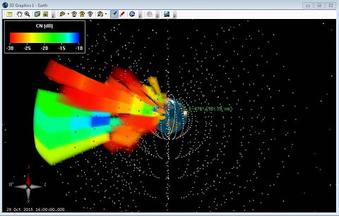
Configure the Graphics of the Volume
- Select the 3D Graphics – Volume page and select the Spatial Calculation Levels option.
- Click Insert Evenly Spaced Values... button to set the contour levels to the following values:
- Click the Create Values button.
- Set the Translucency for the first level to 44% and click Apply.
- Select the 3D Graphics – Legends page.
- Enable the Show Legend option.
- Set the title to CN (dB).
- Enter the following values:
- Click Apply.
The min and max values of the spatial calculation are located in the upper-right.
| Option | Value |
|---|---|
| Start | -30 |
| Stop | Round up to the highest Max integer |
| Step | 5 |
| Option | Value |
|---|---|
| Number of Decimal Digits | 0 |
| Color Square Width (pixels) | 50 |
View in 3D
- Bring the 3D Graphics window to the front to view your volumetric coverage results.
- Reset the animation time.
- Click the Home View (
 ) then zoom out so you can see the whole airspace.
 - Save () your scenario.
To animate your scenario, Volumetric will need to recompute the data at every time step. In order to compute all of the data beforehand to animate smoothly, adjust the Volumetric - Interval to use the "At times at step size" option, and set as desired.
Model a hosted payload on the communication satellites to track a Geosynchronous satellite using EOIR
This section requires an EOIR license and a separate EOIR installation. Please contact us for assistance.
In addition to providing communications, you would like to analyze the performance of a hosted EOIR payload on the LEO communication satellites that would track other satellites.
Save STK11_EOIR as a New Scenario
- Extend the File menu.
- Click the Save As option.
- In the Save As pop up window, click STK User.
- Click the Create New Folder button.
- Name the new folder STK11_EOIR.
- Click Open.
- Change File Name to STK11_EOIR and click Save.
Model the GeosynchronousTarget Satellite
You will be using a representative Geosynchronous satellite as the target for your analysis
- Bring the Insert STK Objects () tool to the front.
- Insert and Satellite object () using the Orbit Wizard () method.
- Set the following options:
- Click OK.
| Option | Value |
|---|---|
| Type | Geosynchronous |
| Name | GEO |
| Inclination | 1 deg |
| Color | White |
Configure the EOIR Properties of the Satellite
- Open the properties of the GEO satellite ().
- Go to the Basic - EOIR Shape page, and set the Shape to GEOComm.
- Set the Body Temperature to 300 K.
- Set the Material to Gold MLI.
- Click OK.
You can use the CustomMesh option to browse to a custom model for the EOIR target object.
Insert an EOIR Sensor
- Bring the Insert STK Objects () tool to the front.
- Insert a Sensor object (
 ) using the Define Properties () method.
 - Attach the sensor () to the LEO_Comm_Sat () satellite.
- Set the Sensor type to EOIR.
- Set the Horizontal and Vertical Half Angles to .001 deg.
- Select the Optical tab, then set the Effective Focal Length to 250 cm.
- Select the Radiometric tab, and change the Units for Saturation and Sensitivity to Radiance.
- In the Sensitivity section, set the EquivalentValue to 1e-008 then hit Enter.
- Click Apply.
- Select the Basic - Pointing page.
- Change the Pointing Type to Targeted.
- Move () the GEO Satellite to the Assigned Targets list.
- Select the 3D Graphics - Attributes page, and enable the Show Radial Lines option.
- Click OK and rename the sensor to EOIR.
- Click the Home View () then zoom out so you can see the GEO satellite.
- Reset (
 ) the scenario animation.
Plot the Signal to Noise Ratio
- Extend the View menu and select Toolbars.
- Select the EOIR_Sensor_Plugin toolbar.
- Click the EOIR Configuration () panel.
- Move () the GEO Satellite to the Selected Targets list.
- Click OK.
- Right-click on the EOIR sensor, and open the Report and Graph Manager.
- Right-click the STK11_EOIR_Styles folder, and select New Graph
- Type EOIR_SNR, then hit Enter.
- Expand EOIR Sensor To Target Metrics and double-click Signal to noise ratio add it to the Y Axis.
- Click OK.
- Double-click EOIR_SNR to generate a graph.
- Select the GEO satellite as the target for the graph, then click OK.
- When the graph comes up, right-click at the maximum value, and select Set Animation Time.
- View your 3D graphics window to see where the satellites are with respect to the Sun.
-
Save (
) the Scenario ().
This graph may take a while to calculate.
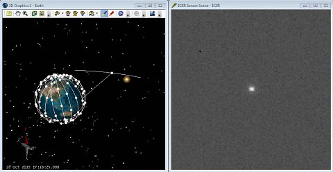
Generate a Synthetic Sensor Scene
- Ensure that the EOIR sensor is selected in the Object Browser, then click the Synthetic Sensor Scene (
 ) button.
 - When the synthetic scene comes up, right-click anywhere in the image and click the Details…option.
- In the Scene Detail field, set the option to Fine.
- Left-click at various locations in the image to determine the spectral Radiance.
- Left-click around the center of the image and note the lower Spectral Radiance for the GEO satellite.
- Save () the Scenario ().
Model LEO satellite Interference
You need to evaluate any interference impacts to the communications link budget between the transmitter on the Geostationary Earth Orbit satellite and the receiver on a ship caused by Low Earth Orbiting satellite's transmitters.
Save STK11_Phased_Array_SATCOM as a New Scenario
- Extend the File menu.
- Click the Save As option.
- In the Save As pop up window, click STK User.
- Click the Create New Folder button.
- Name the new folder STK11_LEOInterference.
- Click Open.
- Change File Name to LEOInterference and click Save.
To begin this section without completing the previous sections, Launch STK and Open a Scenario using the agi.com Scenarios option. Navigate to STK Data Federate Server/Sites/AGI/documentLibrary/STK11/What’s New Scenarios/PhasedArray and open STK11_NewFeaturesTutorial_PhasedArray_SATCOM.vdf. Make sure to Save this as a .sc file in your user directory.
Clean up the Scenario
- Turn Vol_CN off in the Object Browser.
- Save the .sc file.
- Delete the LEO_Comms_Sats Constellation ().
- Click Yes on the pop up window asking if you want to delete the assigned objects too.
This will remove the LEO_Comm_Sat satellites previously set up using the Walker tool. We will recreate this Walker Constellation to include the new LEOXmtr on each satellite.
Geostationary Satellite
Use the Orbit Wizard to insert a Geostationary satellite into the scenario.
- Use the Insert STK Objects tool to insert a Satellite object using the Orbit Wizard method.
- Change Type: to Geosynchronous.
- Change the Satellite Name to GEOSatellite.
- Click OK.
Model the GEOSatellite Transmitter Equipment
You have the scenario level objects in your scenario. Now you can focus on modeling the GEOSatellite transmitter. Build the transmitter.
- Insert a Transmitter object () using the Define Properties () method.
- When the Select Object window appears, select GEOSatllite () in the list and click OK.
- On the Basic - Definition page, make the following change:
- Click Apply.
- Select the Basic - Definition page.
- Click the Modulator tab.
- Enable the Use Signal PSD,
- Set the Number of Spectrum Nulls to three (3).
- Click Apply.
| Option | Value |
|---|---|
| Type: | Complex Transmitter Model |
| Power: | 32 dBW |
Antenna Orientation
Orient the Gaussian antenna on the GEOSatellite to the DDG ship. In this case, the antennas have a fixed boresight.
- Select the Basic – Definition page.
- Click the Antenna tab.
- Click the Orientation tab.
- Set the following changes:
- Click OK to accept change.
- Close the Properties browser.
- Rename the Transmitter object "GeoXmtr."
| Option | Value |
|---|---|
| Azimuth: | 236.701 deg |
| Elevation: | 84.059 deg |
Place the Transmitter into a Constellation
Put the GeoXmtr into the SATCOM_Tx Constellation object.
- Open SATCOM_Tx Constellation's () Properties ().
- Remove any other objects from the SATCOM_Tx constellation.
- Move () GeoXmtr from the Available Objects list to the Assigned Objects list using the right arrow.
- Click OK to accept changes and close the properties browser.
Build a DDG Receiver
The Receiver object is attached to the DDG ship object.
- Insert a Receiver () object using the Define Properties () method.
- When the Select Object window appears, select DDG in the list.
- Click OK.
- Select the Basic – Definition page.
- Set the Type: to Complex Receiver Model.
- Disable Frequency Auto Track.
- Ensure the Frequency is set to 14.5 GHz.
Set the Filter Options
- Select the Filter tab.
- Disable the Bandwidth Auto Scale.
- Set the Bandwidth to 96 MHz.
- Click Apply.
Set the Antenna to Phased Array
- Select the Antenna tab.
- Set the following options:
- Select the Beam Direction Provider tab.
- Enable Beam Steering.
- Move () GeoSatellite.
- Click Apply.
| Option | Value |
|---|---|
| Type: | Phased Array |
| Number of Elements X: | 5 |
| Number of Elements Y: | 5 |
Display the Volume Graphics
- Select the 3D Graphics - Attributes page.
- Enable Show Volume for the Volume Graphics. Keep the default values.
- Click OK to accept the changes and close the properties browser.
- Rename the Receiver object DDG_PA_Rx ().
Add a Vector
- Disable the DDG_PA_Radar () object in the Object Browser.
- Open DDG ship's () properties ().
- Select the 3D Graphics - Vector page.
- Disable the DDG_To_X-47B Vector.
- Click Add... to open the Add Components window.
- Select DDG on the left, expand the To Vectors folder on the right.
- Select the GEOSatellite.
- Click OK.
- Click OK to apply changes and dismiss the properties browser.
View DDG in the 3D Graphics window
- Right-click on DDG in the Object Browser.
- Select Zoom To to view DDG in the 3D Graphics window.
DDG Receiver Constellation
Place the Receiver object into the SATCOM_Rx Constellation object.
- Open SATCOM_Rx Constellation's () properties ().
- Remove any other objects from the SATCOM_Rx constellation.
- Move () DDG_PA_Rx () receiver to the Assigned Objects list.
- Click OK to accept changes and close the properties browser.
GEOSatllite Link Budget
A Link Budget Report between the DDG Receiver and the GEOSatellite Transmitter is simple to accomplish in STK. In this case, the ship is linked to one satellite, therefore, you will perform one link budget per communication link.
- In the Object Browser, right click on DDG_PA_Rx Receiver () and select Access (). This opens the Access Tool.
-
STK allows you to determine the times one object can "access," or see, another object. When the Access Tool opens, at the top where is says “Access for…” the object showing is where you’re looking from. Below that in the Associated Objects List, any objects you choose are objects you’re looking at. By left clicking on the DDG_PA_Rx Receiver and selecting Access, you automatically placed the DDG_PA_Rx Receiver in the Access for… field.
In the Associated Objects List, expand () GEOSatellite (). - Select GeoXmtr ().
- In the lower right hand corner of the Access Tool, in the Reports field, click Link Budget.
This is a simple link budget which can provide some basic information on the performance of your communication link. For the purposes of this lesson, you’ll focus on the Bit Error Rate (BER) column.
- Scroll to the right of the report and note the BER values. For the purpose of this scenario, a BER around 1.000000e-008 or lower will be considered reasonable.
- Close the report and the Access Tool.
Sensor Field of View for Situational Awareness
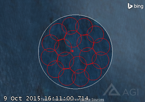
Use a Sensor object’s field of view which will encompass eighteen (18) antenna beams for a particular LEO satellite. This field of view is strictly for operator situational awareness.
- Insert a Sensor () object using the Define Properties () method.
- When the Select Object window appears, select LEO_Comm_Sat in the list.
- Click OK.
- Select the Basic - Definition page.
- Set the following options:
- Click OK to accept changes and close the properties browser.
| Option | Value |
|---|---|
| Sensor Type: | Simple Conic |
| Cone Half Angle: | 2.8 deg |
LEO Transmitter
Each LEO_Comm_Sat satellite has eighteen (18) user transmitter beams. In STK you have choices on how to simulate this configuration. In this tutorial, you’ll use the Multibeam Transmitter Model.
- Insert a Transmitter () object using the Insert Default () method.
- When the Select Object window appears, select LEO_Comm_Sat () in the list.
- Click OK.
- Rename the Transmitter object "LeoXmtr."
Define LeoXmtr's Properties
- Open LeoXmtr's () properties ().
| Option | Value |
|---|---|
| Type | Multibeam Transmitter Model |
| Beam Specs Frequency | 14.51 GHz |
Set the Modulator Options
- Select the Modulator tab.
- Enable the Use Signal PSD.
- Set the Number of Spectrum Nulls to three (3).
- Click Apply.
- Select the Beams tab.
- Select the Antenna tab.
- Select the Orientation tab.
- Set the following changes:
- Click Apply.
| Option | Value |
|---|---|
| Azimuth: | 0 deg |
| Elevation: | 89 deg |
Define the Beams
- In the Beams Selection Table at the top, click on Beam001 in the list.
- Click the Duplicate button seventeen (17) times so that you have a total of eighteen (18) Beams in the list.
- Select Beam001, hold down the Shift key and click on Beam006.
- Click the Orient button.
- Set the following values in the Antenna Beam Orientation panel:
- Click OK.
- Select Beam007, hold down the Shift key and click on Beam018.
- Click the Orient button.
- Set the following values in the Antenna Beam Orientation panel:
Orientation Initial Value Increment Value Elevation: 88 deg 0 deg Azimuth: 0 deg 30 deg - Click OK.
- Click Apply.
| Orientation | Initial Value | Increment Value |
|---|---|---|
| Elevation: | 89 deg | 0 deg |
| Azimuth: | 0 deg | 60 deg |
You can generate an Antenna Properties report for the LEOXmtr to double-check the Beam values match the table below
| Beam ID | Azimuth | Elevation |
|---|---|---|
| Beam001 | 0 deg | 89 deg |
| Beam002 | 60 deg | |
| Beam003 | 120 deg | |
| Beam004 | 180 deg | |
| Beam005 | 240 deg | |
| Beam006 | 300 deg | |
| Beam007 | 0 deg | 88 deg |
|
Beam008 |
30 deg | |
| Beam009 | 60 deg | |
| Beam010 | 90 deg | |
| Beam011 | 120 deg | |
| Beam012 | 150 deg | |
| Beam013 | 180 deg | |
| Beam014 | 210 deg | |
| Beam015 | 240 deg | |
| Beam016 | 270 deg | |
| Beam017 | 300 deg | |
| Beam018 | 330 deg |
Model the Walker Constellation Based on the Template Satellite
You want to model the LEO_Xmtr on each of the LEO_Comm_Sats. You will remove the current LEO_Constellation and thus remove all the satellites, then recreate the Walker Constellation to include the transmitters on each satellite.
- Right-click on LEO_Comm_Sat () in the Object Browser.
- Extend the Satellite menu.
- Select the Walker... option.
- Set the following values:
Option Value Type Custom Number of Sats Per Plane 10 Number of Planes 10 True Anomaly Phasing 60 deg RAAN Increment 18 deg Color by Plane Off Create unique names for sub-objects On Create Constellation On Name of Constellation LEO_Comm_Sats - Click the Create Walker button.
- Click Close once the satellites have all been created. This replicates the multibeam transmitter on each of the LEO_Comm_Sat satellites.
LEO Transmitter Constellation
Group all of the LEO Transmitter objects into a Constellation object.
- Insert a Constellation () object using the Define Properties () method.
- In the Selection filter: enable Transmitter.
- Move () all Transmitter () objects to the Assigned Objects list.
- In the Assigned Objects list, select X47_Tx, GeoXmtr, and LEOXmtr.
- Remove (
 ) these Transmitter objects from the Assigned Objects list.
 - Click OK to accept changes and close the properties browser.
- Rename the Constellation object “LEOInterference."
Interference
In STK, you will use the Comm System object to compute possible communication interference. During the course of the tutorial, you combined the GEOSatellite Transmitter object, DDG Receiver object, and LEOSatellite Transmitter objects into separate Constellation objects. The Comm System object requires this.
CommSystem
- Open the CommSystem's () properties ().
- On the Basic - Transmit page, ensure the SATCOM_Tx is in the Assigned Constellations field. If it is not, move it from the Available Constellations to the Assigned Consolations field.
- Select the Basic - Receive page.
- Ensure the SATCOM_Rx is in the Assigned Constellations field. If it is not, move it from the Available Constellations to the Assigned Consolations field.
- Select the Basic - Interference page.
- Move () the LEOInterference constellation from the Available Constellations to the Assigned Consolations field.
- Click OK to accept changes and close the properties browser.
Compute Interference
You are now ready to determine if the LEO Transmitter objects are interfering with GEOSatellite communication links.
- Save () the scenario. Be patient. This may take a few seconds or a minute due to the amount of objects in the scenario.
- Right-click on the CommSystem ().
- Extend CommSystem menu.
- Click Compute Data.
- Bring the 2D Graphics window to the front. If you do not have a 2D Graphics Window open, click View on the Menu bar and select New 2D Graphics Window. You can see access lines between the DDG Receiver object and the GEOSatellite Transmitter object in the scenario.
- Click the Start (
 ) button in the Animation Toolbar to view these links dynamically.
 - When finished, click the Reset () icon in the Animation Toolbar.
In the lower right hand corner of STK, you will see a progress bar. Wait until the computation is complete.
If the LEO_Comms_Sats ground tracks are cluttering your 2D Graphics Window, multi-select the LEO_Comm_Sats in the Object Browser and right-click to open their Properties. Select the 2D Graphics – Attributes page, deselect Inherit from Scenario, deselect Show Ground Track, and click OK to accept changes and close the properties browser.
View the DDG Ship in 3D
- Bring the 3D Graphics window to the front.
- Zoom To the DDG ship () and look at the access line between the DDG Receiver object and the GEOSatellite Transmitter object.
- Click the Start () button in the Animation Toolbar to view these links dynamically.
- When finished, click the Reset () icon in the Animation Toolbar.
LEO Interference Analysis
Use the Report & Graph Manager to determine if RF interference is affecting the DDG Ship.
- In the Object Browser, right-click on the CommSystem ().
- Select Report & Graph Manager.
- Ensure the Object Type: is set to the Comm System object and CommSystem is selected in the Object List.
- Disable the Show Reports options.
- Enable the Show Graphs options. This cleans up the Styles list and makes it easier to find reports.
- In the Installed Styles folder, right-click the Carrier to Noise vs. Time graph.
- Click Properties ().
- In the Y2 Axis, select Link Information-C(N+I) and remove it.
- Ensure it is selected in the Data Providers list and move it to the Y Axis.
- Click OK.
- Select the new Graph in the My Styles folder and click Generate.
- Update the Step size to one (1) sec.
- Draw a box with your mouse around one of the dips in the graph to Zoom In on that period.
- Right-click on the graph and select Show Animation Time Line.
- Right-click on one of the dips in the graph and select Set Animation Time.
- Zoom To the DDG Ship and zoom out until you can see which LEO Comm satellite is causing the interference. It is LEO_Comm_Sat0903.
For the most part, the link isn’t experiencing very much interference, but if you look closely, there are times that the link does experience interference which is well below the C/N threshold.
Visualize the Beams
You can view the beams in both the 2D and 3D Graphics windows.
- Open properties () of the LEO Transmitter () on LEO_Comm_Sat0903 (LEOXmtr83) ().
- Select the 2D Graphics - Contours page.
- Enable Show Contour Graphics.
- In the Level Adding field, make the following changes:.
- Click Add Level.
- Change the Start Color to red and thicken the Line Width.
- Enable Set azimuth and elevation resolution together.
- Change the Azimuth Resolution to one (1) deg.
- Click Apply.
| Option | Value |
|---|---|
| Start: | -3 |
| Stop: | 0 |
| Step: | 3 |
Enable Contour Graphics
- Select the 3D Graphics - Attributes page.
- In the Contour Graphics, enable Show Lines.
- Click OK to accept changes and close the properties browser.
- Disable the SATCOM_Rx83 () transmitter on LEO_Comm_Sat0903 () in the Object Browser.
View in 3D
- Bring the 3D Graphics window to the front.
- Zoom To LEO_Comm_Sat0903 ().
- Use the left and right mouse buttons to move your view. You can see the antenna beams crosshairs inside the simple conic sensor’s field of view. At this time the ship is directly in the center of the beam and interference is high.
- When finished, close all reports and the Report & Graph Manager.
- Save () the scenario.
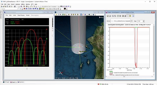
Spectrum Analyzer
- Click on View on the Menu bar.
- Extend the Toolbars menu.
- Select Spectrum Analyzer.
- Click on the Spectrum Analyzer icon in the Toolbars section of the GUI.
- In the Spectrum Analyzer window, select GEOXmtr () and LEOXmtr83 () on LEO_Comm_Sat0903 in the Transmitters section.
- Right-click on LEOXmtr83 ().
- Set the color to red and click OK.
Enable the Receiver View
- Enable the Receiver View.
- Ensure the Lock To Receiver option is selected.
- Set the Vertical Scale to -160.
Enable the Data Display
- Select Data Display on the Spectrum Analyzer Menu bar.
- Ensure Peak and C/I are selected.
- Extend the Edit menu on the Menu bar.
- Click Properties...
- Update the Sweep Line Width to three (3).
- Click Ok.
Enable the Time Step
- Open the 3D Graphics Window properties ().
- Select the Annotation tab.
- Enable the Show Time Step option.
- Click OK.
- Increase () the animation time step to three (3) sec.
- Play () the scenario and watch the interference dominate the desired signal for a short amount of time.
- Save () your scenario.
 Visit AGI.com