Performing Design of Experiments Using Analyzer
STK Pro, Coverage, Analyzer
Additional installation - Analyzer. Contact Support at 1-800-924-7244 to request Analyzer and the Analyzer license.
Analyzer
Analyzer is integrated into the STK workflow to help you automate and analyze STK trade studies to better understand the design of your system.
Using Analyzer, Scenario parameters can be systematically modified to learn more about your Scenario. For purposes of this tutorial, Analyzer will be used to:
- Perform Trade Studies. Analyzer will allow you to quickly perform “what if” studies so that you can understand how changing various Scenario parameters will impact the Scenario.
- Optimize Scenario Parameters. Once you understand the key parameters of a Scenario, an optimizer will be employed to drive the Scenario to an optimal configuration.
For more information on Analyzer, see www.agi.com.
Tutorial
In this tutorial, you will do the following:
- Analyze a STK Scenario for trends.
- Use the Design of Experiments tool
This tutorial is designed to teach you how to use Analyzer’s Design of Experiments tool to vary two or more parameters in your scenario and observe the impact on an output.
Starter Scenario
To speed things up and allow you to focus on the portion of this exercise that teaches you Analyzer, a partially created scenario has been provided for you.
Load the Starter Scenario
To open the scenario:
- Ensure that the Welcome dialog is visible in the STK Workspace.
- Click the Open a Scenario button, select agi.com Scenarios from the left side of the Welcome dialog, and browse to:
Sites/AGI/STK 11/ Started Tutorials/...
- Open the Node Height Scenario (NodeHeight.vdf).
Save the Starter Scenario as an*.sc File
When you open the scenario, a folder with the same name as the scenario will be created in the default user folder (C:\Documents\STK 11 (x64), for example). The scenario will not be saved automatically. When you save a scenario in STK, it will save in the format in which it originated. Therefore, if you open a VDF, the default save format will be a VDF. The same is true for a scenario file (*.sc). To save the VDF as an SC file, change the file format using the Save As procedure:
- Open the File menu and select Save As...
- Click
 to browse to your user location.
 - Click the New folder button (
 ) and give it the same name as the scenario.
 - Open the newly created folder.
- Change Save as type: to Scenario Files (*.sc) and click Save.
Project: Communication Nodes
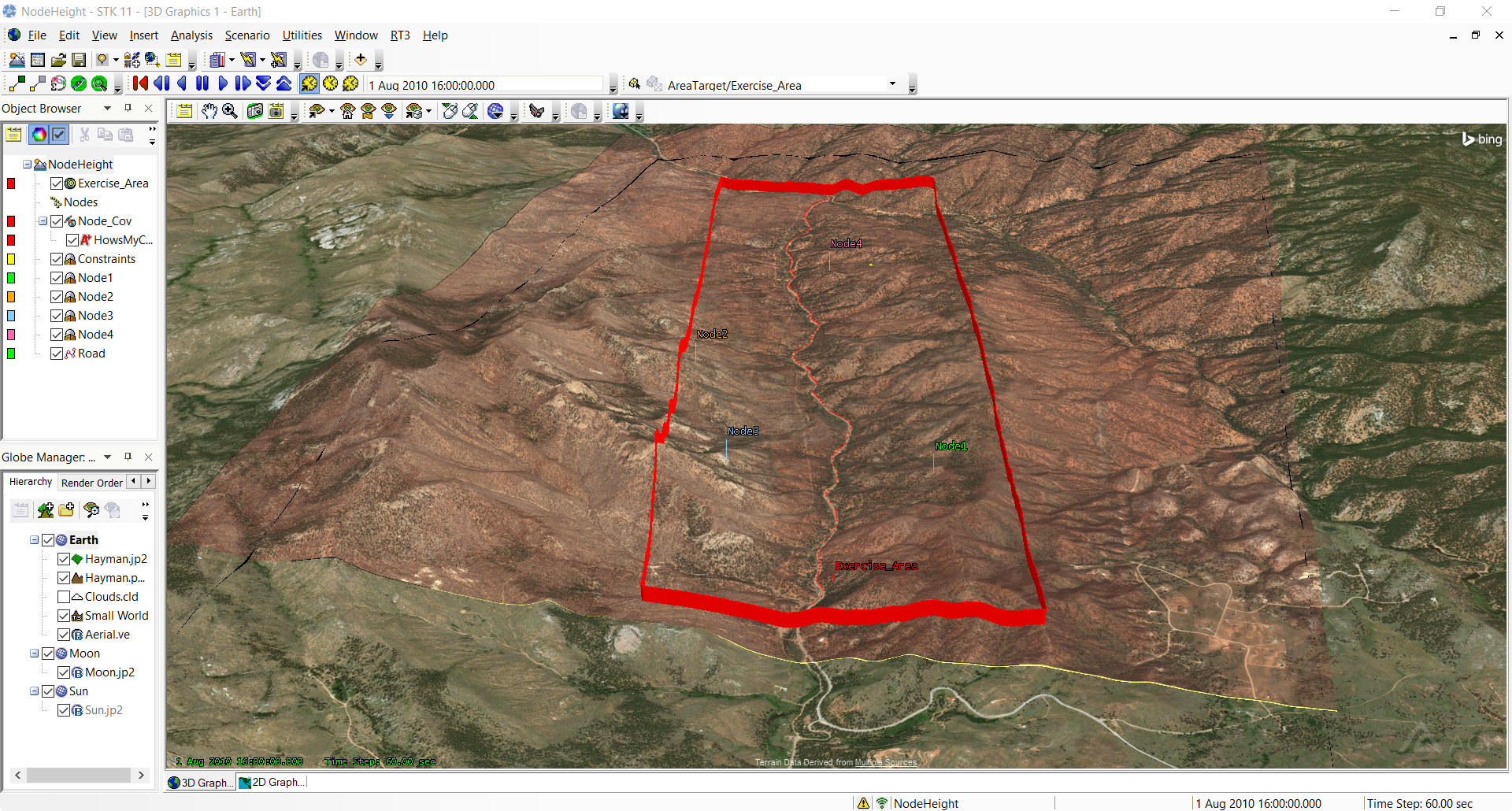
The goal of this project is to study the impact of terrain on a communications link to a vehicle traveling on a road through the mountains. There are four proposed locations for communication nodes that would be used as relays to a satellite and finally to a receiving station. We would like to assess the impact of antenna height on the ability to communicate with a vehicle on the road.
We will first create a carpet plot to see the impact of changing two antennas at a time. We will then use the design of experiments tool to vary the height of all four antennas at the same time so that we can find the best possible configuration for all the antennas.
Exercise 1. Compute Coverage Statistics
We will use Analyzer to perform studies on the Percent Satisfied report for a Figure of Merit. To understand this report, data will first be manually collected in STK.
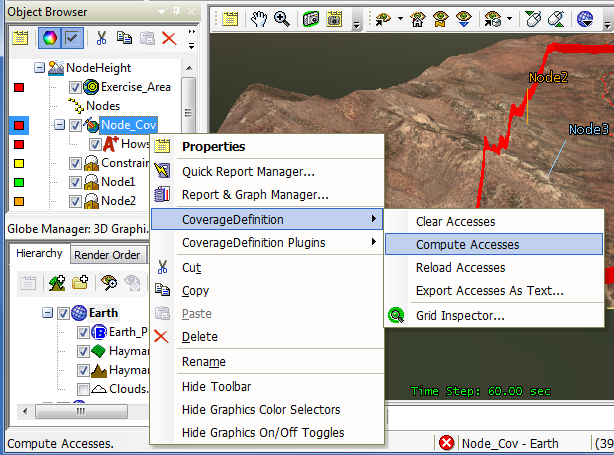
- Compute accesses for the Node_Cov coverage area.
- Right-click on Node_Cov in the Object Browser.
- Expand CoverageDefinition in the context menu.
- Select Compute Accesses.
- Generate a Percent Satisfied report in STK.
- Right-click on the HowsMyCov Figure of Merit (FOM) under the Node_Cov object in the Object Browser.
- Select the Report and Graph Manager... menu item.
- Expand the Installed Styles folder.
- Generate a Percent Satisfied report.
In the resulting report, note the % Satisfied value. This value will be accessible in Analyzer as an output variable.
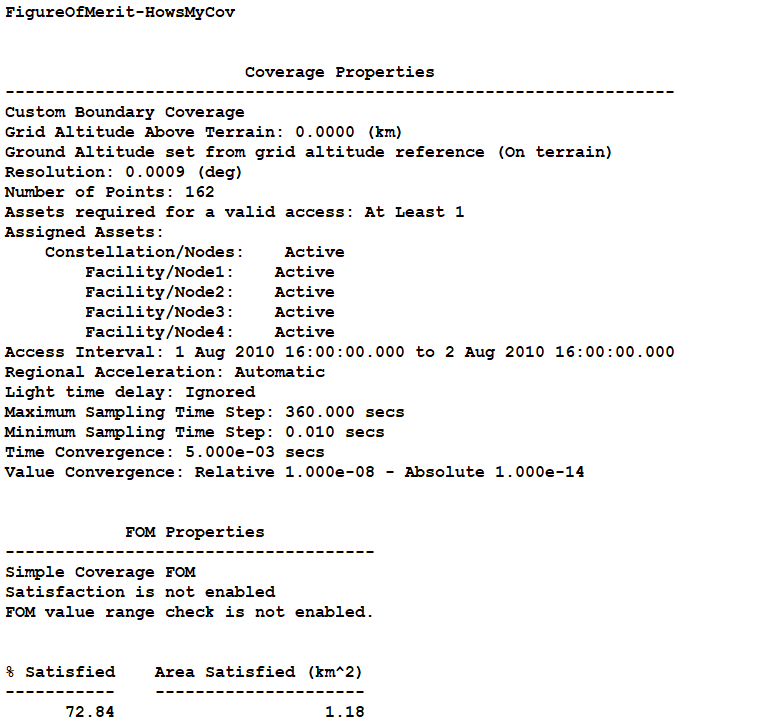
With all of the antennas at ground level, the proportion of the route that is covered is about 73%.
Exercise 2. Open Analyzer
- Click View on the Menu bar.
- Extend the Toolbars menu.
- Select Analyzer. This will bring up the Analyzer toolbar.
- Click on the Analyzer icon (
 ) to bring up the main Analyzer window. This is where input and output variables of the scenario may be selected to analyze.
Exercise 3. Assess the Impact of Changing Two Antenna Heights
We will first run a carpet plot to analyze the impact of raising the height of two of the antennas. We could choose any pair of antennas we would like. For this study, we will look at Node1 and Node3.
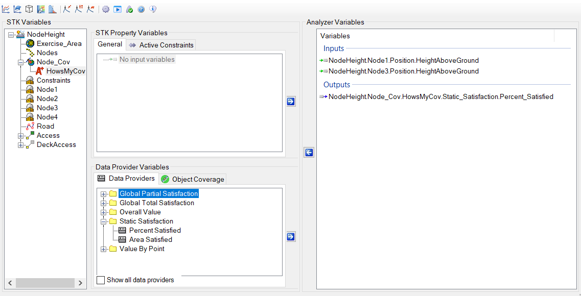
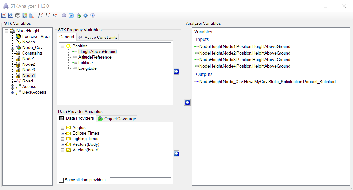
From the Analyzer main form, we will add input and output Analyzer variables.
- Select the input Analyzer variables for this trade study.
- In the STK Variables list, select Node1.
- In the STK Property Variables field, extend Position.
- Click and drag HeightAboveGround to the Analyzer Variables section or select HeightAboveGround and move (
 ) it to the Analyzer Variables section. It will show up under the Inputs list.
 - Repeat the steps above to move Node3 HeightAboveGround to the Analyzer Variables Inputs section as well.
- Select the output Analyzer variables for this trade study.
- In the STK Variables list, expand Node_Cov, and select the HowsMyCov FOM.
- In the Data Provider Variables section, expand Static Satisfaction.
- Click and drag Percent Satisfied to the Analyzer Variables section or select Percent Satisfied and move () it to the Analyzer Variables section. It will show up under the Outputs list.
- In the Analyzer window, click on the Carpet Plot icon (
 ) to open a new Carpet Plot study.
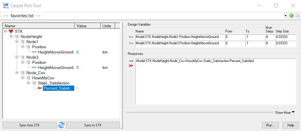
 - Fill in the Design Variables (input variables):
- Under Node1 > Position, click HeightAboveGround in the Component Tree on the left, and drag it to the input field on the right.
- Under Node3 > Position, click HeightAboveGround in the Component Tree on the left, and drag it to the input field on the right.
- Set the following values for both inputs:
Option Value From: 0 To: 0.1 number of samples: 4 step size: 0.03333 - Fill in the Responses (output variables):
- Click on Percent_Satisfied in the Component Tree on the left.
- Drag it to the Responses field on the right.
- The Carpet Plot study should look like this:
- Perform the carpet plot by pressing the Run… button. Note that no plots will appear for this study until all data points have been collected.
Once the trade study is complete and all data has been collected, the Data Explorer toolbar becomes active. 
There are multiple views that can be selected to visualize the data seen on the Table Page. You can choose views by clicking on Add View. You can build custom views or switch to Legacy Views.
- Close the 2D Scatter Plot that opened when you ran the trade study.
- On the Table Page tool bar, expand Add View and select Legacy Views.
- On the Legacy Data Explorer page, expand Standard Plots.
- Select the 3D Surface Plot.
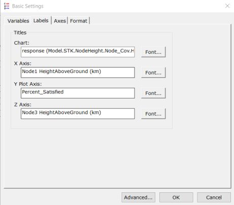
- Since both variable names are the same (HeightAboveGround), it’s hard to distinguish which is which on the plot. We can change the labels in the chart settings. Click Chart on the menu bar, and select Basic Settings. The X axis corresponds to the first design variable (Node1) and the Z axis corresponds to the second design variable (Node3). We could check the Variables tab to confirm this if desired. Set the X and Z axis labels as shown below.
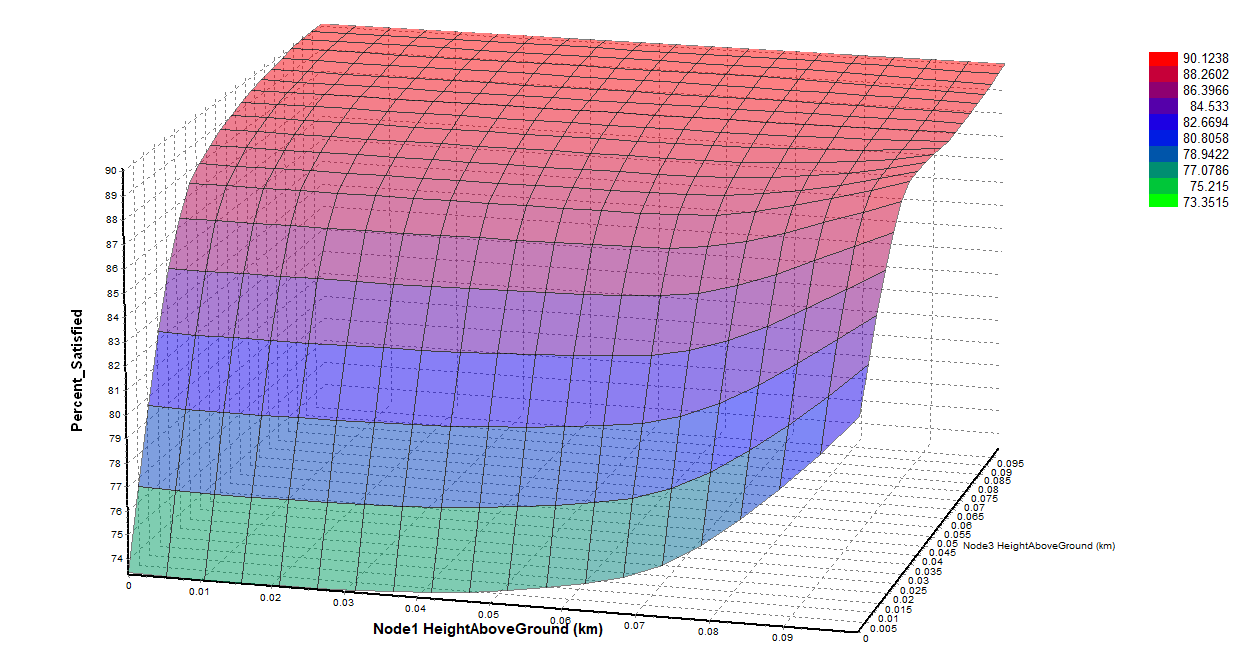
- The new plot is shown below.
- Now create a Contour Plot.
- On the Legacy Data Explorer page, expand Standard Plots.
- Select the Contour Plot.
- Both variable names are again the same (HeightAboveGround) making it hard to distinguish which is which on the plot. Click Chart on the menu bar, and select Basic Settings. The X axis corresponds to the first design variable (Node1) and the Z axis corresponds to the second design variable (Node3). Set the X and Z axis labels as shown below.
- The new plot is shown below.

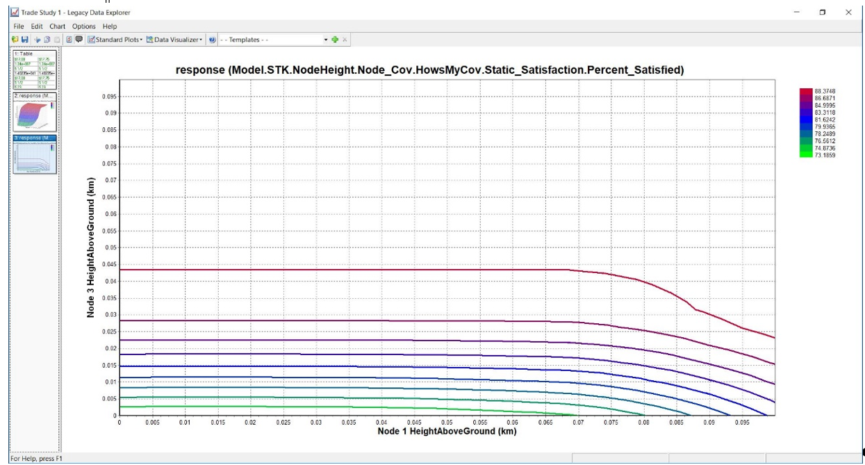
- The 3D Surface Plot and Contour Plot indicate that changing Node3’s height has a much greater impact on the percent of the road covered than Node1.
The Carpet Plot gives a valuable way to visually analyze the impact of two variables on coverage capabilities. However, we would still like to see the impact of varying the height of all of the nodes. The Design of Experiments tool will allow us to do this.
- Close the Trade Study - Legacy Data Explorer page.
- Close the Table - Trade Study - Data Explorer page.
- When prompted to save, select No.
- Close the Carpet Plot Tool window.
Exercise 4. Vary All Four Antenna Heights Using Design of Experiments
We’ve seen the impact of varying two antenna heights. The carpet plot showed that varying Node1’s height had less impact on coverage time than varying Node3’s height. By using the Design of Experiments tool, we’ll be able to see how each of the nodes impact coverage time.
- On the Analyzer main form, add HeightAboveGround for Node2 and Node4.
- In the STK Variables list, select Node2.
- In the STK Property Variables field, extend Position.
- Click and drag HeightAboveGround to the Analyzer Variables section or select HeightAboveGround and move () it to the Analyzer Variables section. It will show up under the Inputs list.
- Repeat the steps above to move Node4 HeightAboveGround to the Analyzer Variables Inputs section as well.
- Click on the Design of Experiments (DOE) icon (
 ) on the Analyzer toolbar.
 - Fill in the Design Variables (input variables):
- Under Node1 > Position, click HeightAboveGround in the Component Tree on the left, and drag it to the input field on the right.
- Repeat the step above for Node2, Node3, and Node4.
- Set the following values for all four Design Variables Values:
Option Value Low: 0 High: 0.1 - Fill in the Responses (output variables):
- Click on Percent_Satisfied in the Component Tree on the left.
- Drag it to the Responses field on the right.
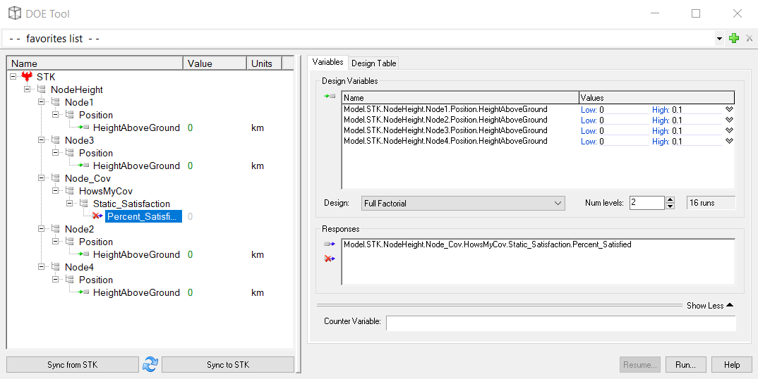
- The DOE Tool should look like this:
- Perform the study by pressing the Run… button.
- Create a Main Effects plot to show the relative impact of each input on the output.
- On the Table Page tool bar, expand Add View and select Legacy Views.
- On the Legacy Data Explorer page, expand Standard Plots.
- Select the Main Effects.
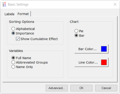
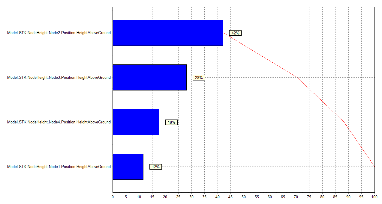
- The labels include only HeightAboveGround and not the name of the Node. Click Chart on the menu bar, and select Basic Settings. Go to the Format tab, and select Full Name under Variables, as shown below. Click OK to confirm the settings.
After examining the table of results, we can see that the best possible coverage percentage is 95%. It is interesting to note that this amount of coverage can be achieved with only two antennas raised to 100 m. This occurs with the combination of Node1 and Node2 as well as the combination of Node2 and Node3, each raised to 100 m.
The Main Effects plot shows the relative impact of each input on the output. As can be seen in the plot, Node2 and Node3 have the most impact on coverage.
 Visit AGI.com