Analyzer: Radar Analysis
STK Pro, Radar, Analyzer
Additional installation - Analyzer. Contact Support at 1-800-924-7244 to request Analyzer and the Analyzer license.
Analyzer
Analyzer is integrated into the STK workflow to help you automate and analyze STK trade studies in order to better understand the design of your system. For purposes of this tutorial, Analyzer will be used to:
- Parametrically explore the STK design space in order to analyze your radar tracking scenario.
- Perform parameter studies that vary an input variable through a range of values and plot one or more output variables.
Launch Vehicle Tracking Exercise
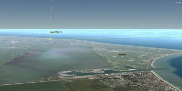
A Launch Vehicle Object will be launched and burns out in ten minutes. A radar site near the launch pad will track the launch vehicle using a phased array antenna.
The goal of this scenario is to study the impact of two variables on the performance of a radar used to track the launch vehicle.
You will run several parametric studies and a carpet plot to gain a better understanding of how these parameters impact performance. In this case, performance will be measured by integrated probability of detection (PDet). You would like for the average integrated PDet to be close to 0.5 to ensure that the radar can track the launch vehicle. Finally, you will use the Optimization Tool to determine the best parameter combination that will provide the highest probability of tracking the launch vehicle. The input parameters you will be studying are:
- Wavelength
- Peak power
You will use base values of 0.1 m for wavelength and 40 dBW for peak power.
Starter Scenario
To speed things up and allow you to focus on the portion of this exercise that teaches you Analyzer, a partially created scenario has been provided for you.
Load the Starter Scenario
To open the scenario:
- Ensure that the Welcome dialog is visible in the STK Workspace.
- Click the Open a Scenario button, select agi.com Scenarios from the left side of the Welcome dialog, and browse to:
Sites/AGI/STK 11/ Started Tutorials/...
- Select Analyzer_RadarAnalysis.vdf.
- Click Open.
Save the Starter Scenario as an*.sc File
When you open the scenario, a folder with the same name as the scenario will be created in the default user folder (C:\Documents\STK 11 (x64), for example). The scenario will not be saved automatically. When you save a scenario in STK, it will save in the format in which it originated. Therefore, if you open a VDF, the default save format will be a VDF. The same is true for a scenario file (*.sc). To save the VDF as an SC file, change the file format using the Save As procedure:
- Open the File menu and select Save As...
- Click
 to browse to your user location.
 - Click the New folder button (
 ) and give it the same name as the scenario.
 - Open the newly created folder.
- Change Save as type: to Scenario Files (*.sc) and click Save.
3D Graphics Window
External Radar Cross Section Files
While setting up and constraining a radar system, Radar allows you to specify an important property of a potential radar target - its radar cross section (RCS). To design a radar system it is essential to be able to describe the target's echo, which is a function of its size, shape and orientation. RCS is defined as the projected area of a metal sphere that would return the same echo signal as the target if it were substituted for the target.
You will be using a custom radar cross section file to define the RCS of the launch vehicle. A file containing this data is included with the scenario. Load this file in the launch vehicle's properties.
- In the Object Browser, open LaunchVehicle's properties.
- Browse to the RF - Radar Cross Section page.
- At the top of the page, turn off Inherit.
- Expand Compute Type: and select External File.
- Click the Filename: ellipses button.
- Select the file Basic_missile_mono.rcs and click Open.
If you click the ellipses button and you're directed to a directory other than the scenario folder, browse to the scenario directory (e.g. C:\Users\<user>\Documents\STK 11 (x64)\Analyzer_Radar_Analysis) and select the .rcs file.
- Click OK.
Compute Access
You will use Analyzer to perform studies on integrated PDet. First, you’ll need to calculate access between the radar and launch vehicle.
- In the Object Browser, right click on PhasedArrayRadar and select Access.
- When the Access Tool opens, go to the Associated Objects List and select LaunchVehicle.
- Click the Report & Graph Manager button.
- When the Report & Graph Manager opens, in the Styles List, select and generate a Radar SearchTrack report.
- Close the report, the Report & Graph Manager and the Access Tool.
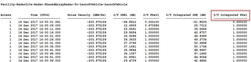
Radar Search Track Results
Note the S/T Integrated PDet value. This value will be accessible in Analyzer as an output variable. The PDet ranges from 0.0001 to 1.0000 with the majority being below the required value of > 0.5000. By varying each of the parameter inputs, you’ll determine which values are necessary to meet the requirement. You’ll also see how a carpet plot will allow you to change more than one input at once and determine what combinations of two inputs can achieve the minimum requirement. The final optimization will provide the best combination of parameters to track the launch vehicle.
Analyzer Layout
The Analyzer Main Form is used to configure input/output variables available for further analysis. You can first select an object in the scenario tree on the left. When an object is selected, all possible input variable candidates are listed under the Inputs General tab and the Inputs Constraints tab. All output variable candidates are listed under the Outputs Data Providers tab, Outputs Object Coverage tab, Outputs DeckAccess tab or Outputs MissileModelingTools tab.
Wavelength Study
The first parameter you will examine is the transmitter's wavelength. You need to select input and output variables from the main Analyzer window to pass to the Parametric Study tool.
Select the input variable.
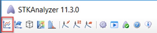
- Click the Analyzer button on the Analyzer Tool Bar.
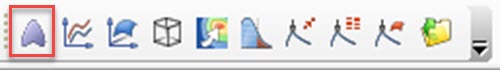
Analyzer Tool Bar Analyzer Icon
Another way of opening Analyzer is to go to the Object Browser, right click on the scenario object (or any object), select the object's Plugins, and click Analyzer.
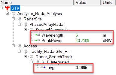
- When Analyzer is open, in the STK Variables list, expand RadarSite.
- Select PhasedArrayRadar.
- In the STK Property Variables field, expand SystemMonostatic.
- Double click Wavelength. This moves Wavelength to the Analyzer Variables field as an input.
Select the output variables.
- In the STK Variables window, expand Access and select Facility-RadarSite-Radar_PhasedArrayRadar-to-LaunchVehicle-LaunchVehicle.
- At the bottom of the Data Providers list, enable Show all data providers.
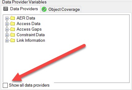
Show All Data Providers
- In the Data Providers field, expand Radar SearchTrack and then S/T Integrated PDet.
- Move Avg into the Analyzer Variables field (double click or use the white arrow in the blue field):
Parametric Study Tool
The Parametric Study Tool is used to run a Scenario through a sweep of values for some input variable. The resulting data can be plotted to view trends.
- In the Analyzer tool bar select Parametric Study.
- When the Parametric Study opens, in the Component Tree, using your left mouse button, drag Wavelength to the Design Variable field on the right.
Parametric Study Icon
Analyzer builds a parametric representation of the currently loaded Scenario. This representation is viewed in the Component Tree displayed on the left side of each trade study tool.
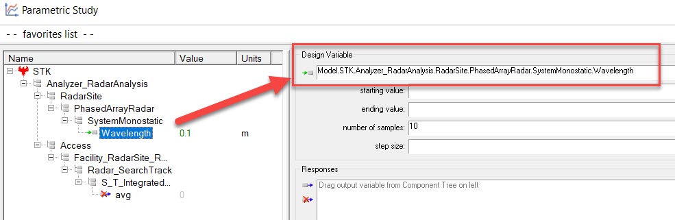
Design Variable
- Set the following Design Variables:
| Option | Value |
|---|---|
| starting value: | .1 |
| ending value: | 5 |
| step size: | .1 |
- In the Component Tree, using your left mouse button, drag Avg to the Responses field on the right.
- In the lower right hand corner of the Parametric Study Tool, click Run.
Data Explorer
The Data Explorer is a tool used by Trade Study tools to display data while they are being collected from STK. While data is being collected, the Data Explorer displays a progress meter, a halt button, and the data.
Table Page
The Table page displays trade study data in a tabular form. It is the default window that is present for all trade studies. Cells are shaded differently depending on the associated variable's state. Input variables are shown with green text, valid values are displayed with black text, invalid values are displayed with gray text, and modified values are displayed with blue text. From the table it is possible to view and edit all values in your trade study and even to add and remove whole runs.
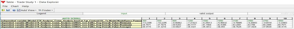
Table Page
The results of your trade studies will show average values throughout.
Toolbar
Once the trade study is complete and all data has been collected, the Data Explorer toolbar becomes active.

Data Explorer Tool Bar
Plot Types
Some trade study tools will automatically launch a default plot window when the trade study runs. Other plots can be created from the Add View dropdown menu.
Views
There are multiple views that can be selected to visualize the data seen on the Table Page. You can choose views by clicking on Add View. You can build custom views or switch to Legacy Views.
- Close the 2D Scatter Plot that opened when you ran the trade study.
- On the Table Page tool bar, expand Add View and select 2D Line Plot.
Dimensions
The Dimensions menu option is used to set which variable is displayed on which axis. In certain plots, other global plot controls can also be set based on the plot variables.
- Click Dimensions.
- Open x pull down menu and select Wavelength.
Axes
The Axes tab is used to set options for the axes.
- Click Axes.
- Select the Ticks tab.
- Change the Max # value to 40.
- Click on the plot to close the Axes menu.
- Close the 2D Line Plot and the Table Page.
- When prompted to save, select No.
- Close the Parametric Study Tool.
- Return to Analyzer.
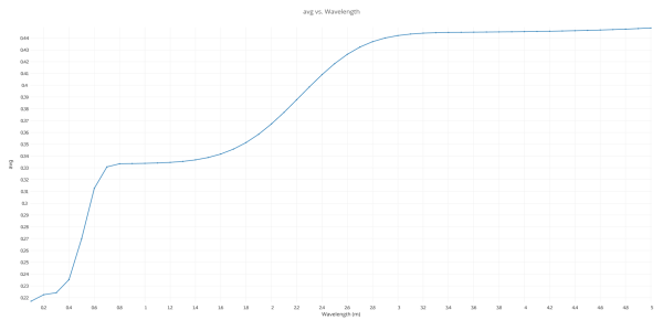
Wavelength 2D Line Plot
As the transmitter's wavelength increases (the frequency becomes lower), the average PDET increases. Between a wavelength of three and five, this increase tapers off.
Peak Power Study
Wavelength is not the only transmitter parameter that will impact your tracking. Peak Power also has an impact. To determine how much, run another Parametric Study.
Select the input variable.
- In the STK Variables list, expand RadarSite.
- Select PhasedArrayRadar.
- In the STK Property Variables field, expand SystemMonostatic.
- Double click PeakPower. This moves PeakPower to the Analyzer Variables field as an input.
- In the Analyzer tool bar select Parametric Study.
- In the Component Tree, using your left mouse button, drag PeakPower to the Design Variable field on the right.
- Set the following Design Variables:
- In the Component Tree, using your left mouse button, drag Avg to the Responses field on the right.
- In the lower right hand corner of the Parametric Study Tool, click Run.
- Close the 2D Scatter Plot that opened when you ran the trade study.
- On the Table Page tool bar, expand Add View.
- Select the 2D Line Plot.
- Change the x dimension to PeakPower.
- Change the Axes Ticks to forty (40).
- Close the 2D Line Plot and the Table Page.
- When prompted to save, select No.
- Close the Parametric Study Tool.
- Return to Analyzer.
| Option | Value |
|---|---|
| starting value: | 40 |
| ending value: | 60 |
| step size: | 1 |
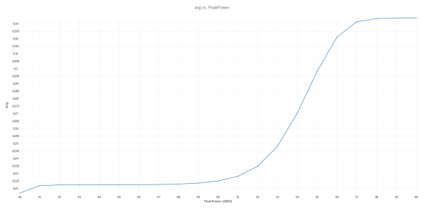
Peak Power Change
Peak Power shows a large average Integrated PDET increase between 50 and 57 dBW.
Determine if Wavelength and Peak Power Impact One Another
You have determined that wavelength and peak power have significant impacts on Integrated PDET. This leads to the following question:
How do wavelength and peak power affect one another?
You can answer the question by performing a 2-dimensional parametric study called a Carpet Plot.
Carpet Plot Tool
A Carpet Plot is a means of displaying data dependent on two variables in a format that makes interpretation easier than normal multiple curve plots. A Carpet Plot can be thought of as a multi-dimensional Parametric Study.
- In the Analyzer tool bar select Carpet Plot.
- In the Component Tree, using your left mouse button, drag Wavelength to the first Design Variable field on the right and PeakPower to the second Design Variable field.
- Set the following Wavelength Design Variables:
- Set the following PeakPower Design Variables:
- In the Component Tree, using your left mouse button, drag Avg to the Responses field on the right.
- In the lower right hand corner of the Carpet Plot Tool, click Run.
- Close the Carpet Plot and the Table Page.
- When prompted to save, select No.
- Close the Carpet Plot Tool.
- Return to Analyzer.
Carpet Plot Study Icon
Setting the design variables is similar to using the Parametric Study Tool except you now have two variables instead of one.
| Option | Value |
|---|---|
| From | .1 |
| To | 5 |
| Num Steps | 10 |
| Option | Value |
|---|---|
| From | 50 |
| To | 60 |
| Num Steps | 10 |
If you are wondering why this tutorial uses large step sizes, it's due to keeping the tutorial time under an hour. These settings will require a total of one hundred runs to obtain every variable combination. On your own, you can set the Wavelength and PeakPower to change at smaller step sizes to make the trade study more realistic. Be patient. Depending on your settings, you could end up running hundreds of runs.
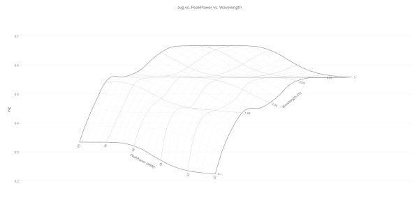
Carpet Plot
Using the Carpet Plot, you can find different combinations of wavelength and peak power that allow you to maintain an average Integrated PDET of .5 or higher.
Optimize Transmitter Parameters
You now know that transmitter parameters have an impact on Integrated PDET. In order to optimize these parameters, you can either guess at values, or employ an optimization tool. Although you can clearly see trends from the previous studies, guessing at values will be difficult because you are dealing with multiple parameters at the same time.
To solve more complex problems, an optimization tool can be a very useful guide. An optimizer is an automated tool that makes mathematical calculations about a design problem and incrementally attempts to find an optimal solution. The algorithm you will employ here is an optimizer. The selected algorithm will compute derivatives about an initial point in the design space and compute a search direction. This process will repeat until no more progress can be achieved on the objective function.
An optimizer will be used in this problem to minimize the peak power requirement for the transmitter while maintaining an average Integrated PDET of ~ 0.5.
Optimization Tool
The Optimization Tool is a collection of optimization algorithms that can be used within Analyzer. Currently over 30 algorithms are available including gradient based optimizers, genetic algorithms, multi-objective algorithms, and other heuristic search methods (see Algorithm Comparison Chart). A common graphical user interface is provided to define optimization problems. An algorithm selection wizard is also provided to make it easy to choose algorithms that will work best for the problem at hand.
- In the Analyzer tool bar select the Optimization Tool.
- In the Component Tree, using your left mouse button, drag PeakPower to the Objective field on the right.
- Ensure Goal is Minimize.
- In the Component Tree, using your left mouse button, drag Avg to the Constraint field on the right.
- Set the Lower Bound to .5 and the upper bound to 1.0.
- In the Component Tree, using your left mouse button, drag Wavelength and PeakPower Design Variables field on the right.
- In the Design Variables field, change the Wavelength Start Value (Explicit Value) to one (1). This value has to be at least or greater than the lower bound value.
- Continue making the following changes:
Optimization Tool Icon
The objective is to minimize the value for peak power by changing wavelength and peak power all while maintaining an average Integrated PDET as close to 0.5 as possible. It's probable that you won't meet your goal due to radar system limitations, but you can still get close.
| Option | Lower Bound | Upper Bound |
|---|---|---|
| Wavelength | 1 | 5 |
| PeakPower | 40 | 60 |
- Set Algorithm to Design Explorer.
- In the lower right hand corner of the Optimization Tool, click Run.
- Close the 2D Scatter Plot.
Design Explorer is an advanced optimization algorithm that was developed to efficiently solve difficult real-world design problems. Design Explorer can effectively solve difficult optimization problems where engineering analyses take long time to run, their responses are noisy and highly non-linear, and engineering simulations may fail. Design Explorer automatically creates approximation models of objectives and constraints and uses them to perform optimization runs with different starting points to find global optimum. Design Explorer solves general constrained optimization problems with continuous design variables.
The optimizer will display a history of steps as it progresses. By default only the objective definition will be displayed.
The above process can be repeated to add plots for frequency and data rate.
When the optimization study is complete, the Table Page will contain the convergence history of the process. The last design point in the Table view will contain the optimized values. These values are also displayed in the Value column for the design variables in the Optimization Tool.
Optimization Values
The Optimization Tool Status reported "Marginal design(s) found. One or more constraints are violated". You weren't able to maintain an average PDET above 0.5. This was due to system limitations. However, the Optimization Tool got you close to the lower bound based on your requirement of using less power.
When You Finish
- Close the Table Page, the Optimization Tool, and Analyzer.
- Save your work.
- Close the scenario.
- Close STK.
 Visit AGI.com