Performing Trade Studies Using Analyzer
STK Pro, Analyzer
Additional installation - Analyzer. Contact Support at 1-800-924-7244 to request Analyzer and the Analyzer license.
Analyzer
Using Analyzer, Scenario parameters can be systematically modified to learn more about your Scenario. For purposes of this tutorial, Analyzer will be used to:
- Perform Trade Studies. Analyzer will allow us to quickly perform “what if” studies so that we can understand how changing various Scenario parameters will impact the Scenario.
- Optimize Scenario Parameters. Once we understand the key parameters of a Scenario, an optimizer will be employed to drive the Scenario to an optimal configuration.
For more information on Analyzer, see www.agi.com.
Tutorial
In this tutorial, you will do the following:
- Analyze a STK Scenario for trends.
- Optimize Scenario parameters to meet mission objectives
This tutorial is designed to teach you how to parametrically explore the STK design space in order to optimize your Scenario. You will learn how to perform parameter studies that vary an input variable through a range of values and plots one or more output variables. You will also learn how to generate 3D surface plots and perform optimization studies.
Project: Polar Ice Cap Exploration
The goal of this project is to launch a satellite into orbit that will be used to monitor icebergs over the polar cap. A LEO satellite will be used to scan the surface. Data will then be relayed through a GEO satellite back to a ground processing facility in Montreal.
The goal for this study is to better understand the requirements for the LEO satellite. In particular this includes specifying orbit parameters for the satellite and configuration of the sensor.
To better understand how the LEO satellite orbit and sensor parameters impact coverage capabilities, a series of parametric studies will be run. For each parametric study, a single design parameter will be run through a sweep of values. At each value, coverage statistics will be collected using a Figure of Merit.
Our goal for this problem is to optimally configure the satellite’s orbit and sensor to best cover the polar ice cap. There are a handful of parameters that will impact our study:
Satellite Orbit:
- Inclination
- RAAN
- Semi-major Axis
Satellite Sensor
- Focal Length
- Detector Pitch
- Ground Sampling Distance
- Cone Angle
To initiate our analysis, we will perform a few parameter studies to see how changing each of these parameters impacts our coverage capability. This will be followed by creation of a carpet plot to view how multiple parameters impact coverage. Lastly, an optimization study will be performed to scan through the design space to find a solution that meets our requirements.
Starter Scenario
To speed things up and allow you to focus on the portion of this exercise that teaches you Analyzer, a partially created scenario has been provided for you.
Load the Starter Scenario
To open the scenario:
- Ensure that the Welcome dialog is visible in the STK Workspace.
- Click the Open a Scenario button, select agi.com Scenarios from the left side of the Welcome dialog, and browse to:
Sites/AGI/STK 11/ Started Tutorials/...
- Open the Sensor Optimization Scenario (SensorOpt.vdf).
Save the Starter Scenario as an*.sc File
When you open the scenario, a folder with the same name as the scenario will be created in the default user folder (C:\Documents\STK 11 (x64), for example). The scenario will not be saved automatically. When you save a scenario in STK, it will save in the format in which it originated. Therefore, if you open a VDF, the default save format will be a VDF. The same is true for a scenario file (*.sc). To save the VDF as an SC file, change the file format using the Save As procedure:
- Open the File menu and select Save As...
- Click
 to browse to your user location.
 - Click the New folder button (
 ) and give it the same name as the scenario.
 - Open the newly created folder.
- Change Save as type: to Scenario Files (*.sc) and click Save.
- Run the Scenario to view the LEO satellite scan the polar ice cap.
Exercise 1. Compute Coverage Statistics
We will use Analyzer to perform studies on the Grid Stats report for a Figure of Merit. To understand this report, data will first be manually collected in STK.
- Compute accesses for the Artic_Monitorcoverage area:.
- Right-click Artic_Monitor in the Object Browser.
- Expand theCoverageDefinitionitem in the context menu.
- SelectCompute Accesses.
- Generate a Grid Stats report in STK.
- Right click CoveragePerDayFigure of Merit (FOM) underArtic_Monitorobject.
- Select the Report and Graph Manager... menu item.
- Expand the Installed Styles folder.
- Generate a Grid Stats report.
In the resulting report, note the Minimum, Maximum, and Average values. These values will be accessible in Analyzer as output variables.
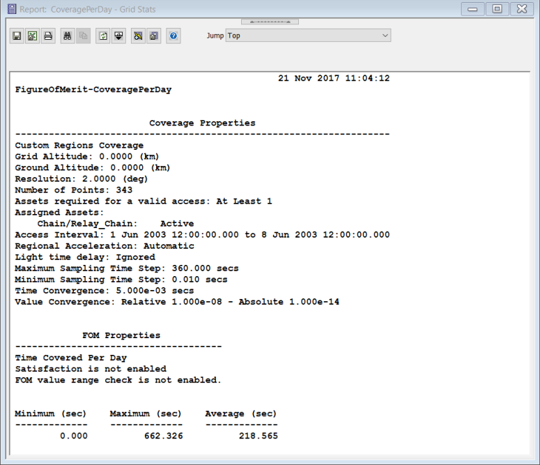
This reports indicates to us that for all the grid points defining the polar cap Coverage Definition, some points are not seen by the satellite at all (Minimum=0), the most any point is seen is 662 seconds per day, and on average points are seen for 219 seconds per day.
Exercise 2. Open Analyzer
- Click View on the Menu bar.
- Extend the Toolbars menu.
- Select Analyzer.
- Click the Analyzer icon (
 ) to bring up the main Analyzer window. This is where input and output variables of the scenario may be selected to analyze.
This will bring up the Analyzer toolbar.
Analyzer imports a copy of the currently loaded Scenario. Any of the STK variables can be added as Analyzer input or output variables. Note that if you change a value of a variable in your Scenario through the STK interface, you should re-add the variable as an Analyzer variable before running any trade studies with the new value.
Exercise 3. Determine the Impacts of Inclination on Coverage
The first study we will perform will vary inclination to determine which values are best.
For this exercise, we will select the inclination as the input variable. The output variables will be average, minimum and maximum coverage per day of the Artic Monitor.
- Select the input Analyzer variables for this trade study.
- In the STK Variables list, select LEO.
- In the STK Property Variables, extend Propagator (J4Perturbation).
- Click and drag Inclination to the Analyzer Variables section or click select Inclination and move (
 ) it to the Analyzer Variables section. It will show up under the Inputs list.
 - Select the output Analyzer variables for this trade study.
- In the STK Variables list, expand the Artic_Monitor Coverage Definition, and select the CoveragePerDay FOM.
- In the Data Provider Variables section, expand Overall Value.
- Click and drag Minimum to the Analyzer Variables section or select Minimum and move () it to the Analyzer Variables section. It will show up under the Outputs list.
- Repeat the previous step for Maximum and Average.
- Select Parametric Study...(
 ) from the Analyzer toolbar.
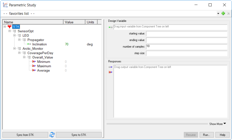
 - Fill in the Design Variable (input variable):
- Click Inclination in the Component Tree on the left.
- Drag it to the input field on the right.
- Set the following values:
Option Value starting value: 45 ending value: 135 number of samples: 10 step size: 10
- Fill in the Responses (output variables):
- Click on Minimum in the Component Tree on the left.
- Drag it to the Responses field on the right.
- Repeat the above steps to add Maximum and Average as additional output variables.
- Perform the parametric study by pressing the Run… button. A Data Explorer window will then appear. The Data Explorer will store and display data from STK for each run in the parametric study. The Table view is used to view actual values returned from STK while the graph views show plots of each of the report variables collected from STK.
- Update the graph to display each Inclination vs the Maximum, Minimum, and Average coverage time.
- In the 2D Scatter Plot window, click on Dimensions (
 ) in the menu list.
 - Click the x drop down box, and select Inclination.
- Ensure Maximum is selected as the y value.
- Click the plus sign at the top of the Dimensions window to create "Series 2".
- Click the x drop down box, and select Inclination.
- Click the y drop down box, and select Minimum. This will change "Series 2" to "Minimum".
- Click the plus sign at the top of the Dimensions window to create "Series 3".
- Click the x drop down box, and select Inclination.
- Click the y drop down box, and select Average. This will change "Series 3" to "Average".
- Select Series (
 ) in the menu on the left.
 - In the Series drop down at the top, select All series (scattergl).
- Select
 as the line marker.
 - Click on the graph to exit out of the menus.
- Return to the Parametric Study window.
- Change the parametric study values to those shown below:
- Perform the parametric study by pressing the Run… button.
- Update the graph to display each Inclination vs the Maximum, Minimum, and Average coverage time.
- In the 2D Scatter Plot window, click on Dimensions () in the menu list.
- Click the x drop down box, and select Inclination.
- Ensure Maximum is selected as the y value.
- Click the plus sign at the top of the Dimensions window to create "Series 2".
- Click the x drop down box, and select Inclination.
- Click the y drop down box, and select Minimum. This will change "Series 2" to "Minimum".
- Click the plus sign at the top of the Dimensions window to create "Series 3".
- Click the x drop down box, and select Inclination.
- Click the y drop down box, and select Average. This will change "Series 3" to "Average".
- Select Series () in the menu on the left.
- In the Series drop down at the top, select All series (scattergl).
- Selectas the line marker.
- Click on the graph to exit out of the menus.
- In the 2D Scatter Plot window, click on Dimensions (
- Close the Parametric Study window.
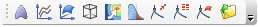
The Parametric Study Tool will appear as shown below:
The tool contains a tree view on the left that lists variables that were selected as Analyzer variables, and that are available from STK for use in the trade study. The fields on the right are used to specify what variables should be used in the study.
Analyzer imports a parametric copy of the currently loaded Scenario. The values currently loaded into Analyzer can be viewed by expanding the tree view to reveal the Value columns.
You will notice multiple icons associated with variables. The  icon indicates that a variable is an input, and may be used as a design variable in a trade studies. The
  icon indicates that a variable is an output, and may be used as a response variable in a trade study. Output variables are computed by STK. Lastly, the
  icon indicates a currently invalid output. This means one of the inputs has changed and Analyzer needs to run again to compute a valid value for the variable. To cause Analyzer to run, click on any of the red X icons.
Analyzer builds a parametric representation of the Scenario each time a trade study tool is loaded. Input values are created for key parameters in the Scenario. Output values are created from reports.
If you change a value in your Scenario through the STK interface, you should re-add the affected variable as an Analyzer variable in the Analyzer window before running the trade study.
The Parametric Study should look like this:
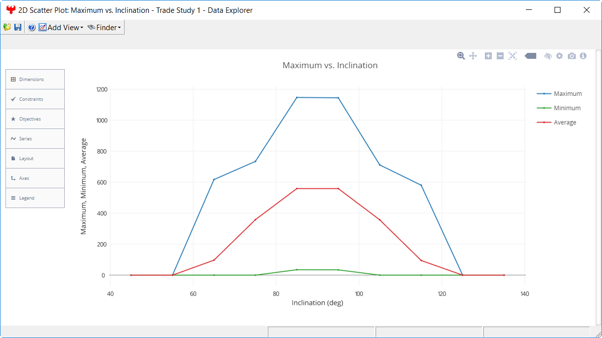
Results from the first study are not unexpected: the closer the inclination is to 90 degrees, the better our coverage capability will be. This makes intuitive sense as the ice cap covers the North Pole and our coverage will be best when our orbit takes us through the rotational center point of the area we are trying to cover.
There are two additional interesting trends in the data. First, maximum coverage does not smoothly improve as inclination approaches 90 degrees. Second, and more importantly, the minimum coverage value does not climb above zero until inclination reaches some value between 75 and 90 degrees.
Since we want to assure that our orbit will cover the entire ice cap, we will run a more refined parametric study in the area of interest.
After running a trade study, Analyzer will reset the values in your Scenario back to what they were before the trade study was started.
| Option | Value |
|---|---|
| starting value: | 75 |
| ending value: | 105 |
| number of samples: | 10 |
| step size: | 3.33333 |
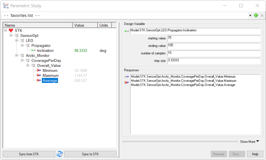
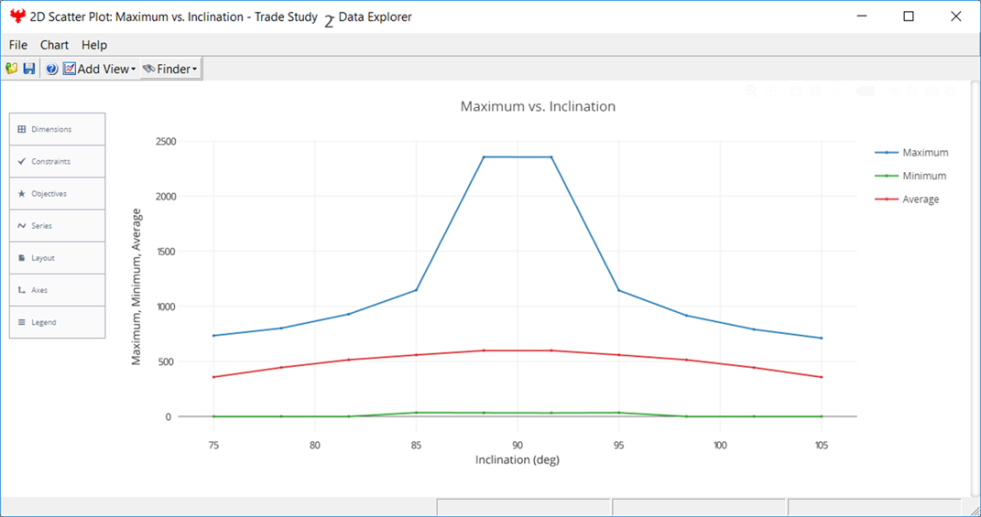
This study gives us a much better understanding of where to position the satellite to give us the best overall inclination to assure maximum coverage of the whole ice cap. We can see that inclinations between 85 and 95 degrees will assure us of at least 32 seconds of coverage per day for each area of the ice cap.
Exercise 4. Determine the Impacts of RAAN on Coverage
Inclination is not the only orbit parameter that will impact our coverage capabilities. RAAN may also have an impact. To determine if it does, we will run another parametric study.
- Now that we have determined interesting values for inclination, change the inclination value to 90 for further studies.
- Right-click on the LEO satellite in the Object Browser, and open its Properties.
- On the Basic-Orbit page, change Inclination to 90 deg, and click OK.
- Return to the Analyzer window, and add RAAN as an input variable.
- In the STK Variables list, select LEO.
- In the STK Property Variables, extend Propagator (J4Perturbation).
- Click and drag RAAN to the Analyzer Variables section or click select RAAN and move () it to the Analyzer Variables section. It will show up under the Inputs list.
- Click on the Parametric Study icon () to open a new Parametric Study.
- Click Sync from STK to update the LEO's Inclination to 90 deg value matching the updated value in STK. Another way to update the value in the Parametric Study is by re-adding the variable as an input in the Analyzer window.
- Fill in the Design Variable (input variable):
Option Value Design Variable (input) RAAN starting value: 0 ending value: 360 number of samples: 10 step size: 40 - Fill in the Responses (output variables).
- Click on Minimum in the Component Tree on the left.
- Drag it to the Responses field on the right.
- Repeat the above steps to add Maximum and Average as additional output variables.
- Perform the parametric study by pressing the Run… button.
- Update the graph to display each RAAN vs the Maximum, Minimum, and Average coverage time.
- In the 2D Scatter Plot window, click on Dimensions () in the menu list.
- Click the x drop down box, and select RAAN.
- Ensure Maximum is selected as the y value.
- Click the plus sign at the top of the Dimensions window to create "Series 2".
- Click the x drop down box, and select RAAN.
- Click the y drop down box, and select Minimum. This will change "Series 2" to "Minimum".
- Click the plus sign at the top of the Dimensions window to create "Series 3".
- Click the x drop down box, and select RAAN.
- Click the y drop down box, and select Average. This will change "Series 3" to "Average".
- Select Series () in the menu on the left.
- In the Series drop down at the top, select All series (scattergl).
- Selectas the line marker.
- Click on the graph to exit out of the menus.
- In the 2D Scatter Plot window, click on Dimensions (
- Create a new graph to view just the minimum coverage values.
- In the 2D Scatter Plot window, clickAdd View, and select2D Scatter Plot.
- In the new 2D Scatter Plot window, click on Dimensions () in the menu list.
- Click the x drop down box, and select RAAN.
- Click the y drop down box, and select Minimum.
- Select Series () in the menu on the left.
- Selectas the line marker.
- Click on the graph to exit out of the menus.
- Close the Parametric Study window.
The Parametric Study should look like this:
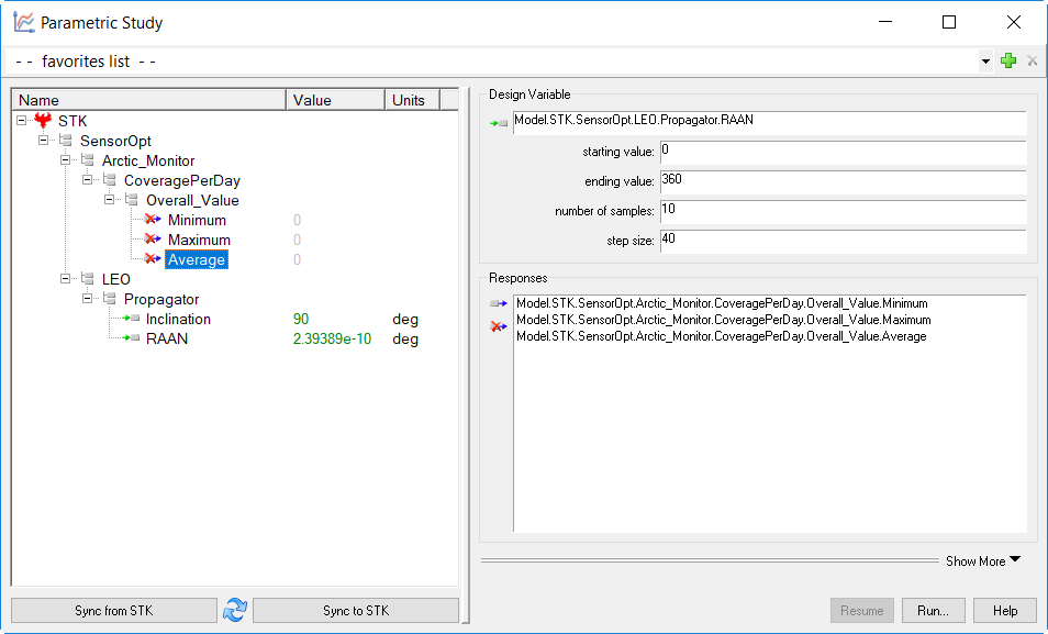
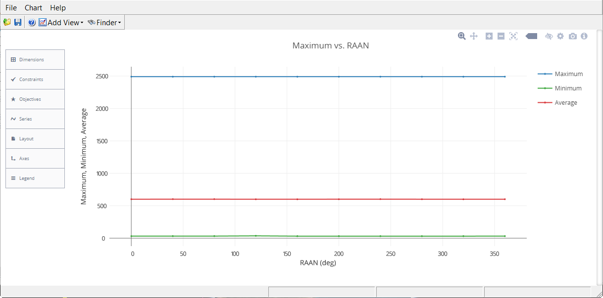
At first glance the data appears to be insensitive to RAAN. This, however, may be due to the difference in scales minimum and maximum coverage values. To view just the minimum coverage values, we will create a new graph.
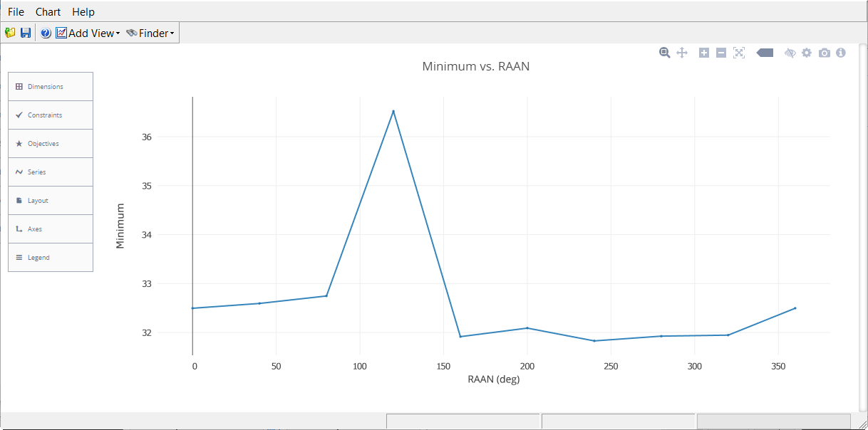
Minimum coverage values seem to fluctuate unpredictably for different RAAN values. This is an artifact of the low frequency sampling of the data. While the difference between high and low values is less than 10 percent of the mean, there are definitely some values that are better than others.
Exercise 5. Determine the Impacts of Altitude on Coverage
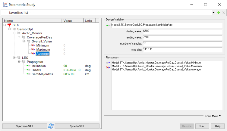
The final orbit parameter impacting coverage is the altitude of the orbit, or expressed in classical orbit parameters, the semi-major axis. For this study, we will vary the orbit from 6,500 km to 7,500 km.
- In the Analyzer window, add semi-major axis as an input variable.
- In the STK Variables list, select LEO.
- In the STK Property Variables, extend Propagator (J4Perturbation).
- Click and drag SemiMajorAxis to the Analyzer Variables section or click select SemiMajorAxis and move () it to the Analyzer Variables section. It will show up under the Inputs list.
- Click on the Parametric Study icon () to open a new Parametric Study.
- Fill in the Design Variable (input variable):
- Click SemiMajorAxis in the Component Tree on the left.
- Drag it to the input field on the right.
- Set the following values:
Option Value starting value: 6500 ending value: 7500 number of samples: 10 step size: 111.111 - Fill in the Responses (output variables):
- Click on Minimum in the Component Tree on the left.
- Drag it to the Responses field on the right.
- Repeat the above steps to add Maximum and Average as additional output variables.
The Parametric Study should look like this:
- Perform the parametric study by pressing the Run… button.
- Update the graph to display SemiMajorAxis vs the Maximum, Minimum, and Average coverage time.
- In the 2D Scatter Plot window, click on Dimensions () in the menu list.
- Click the x drop down box, and select SemiMajorAxis.
- Ensure Maximum is selected as the y value.
- Click the plus sign at the top of the Dimensions window to create "Series 2".
- Click the x drop down box, and select SemiMajorAxis.
- Click the y drop down box, and select Minimum. This will change "Series 2" to "Minimum".
- Click the plus sign at the top of the Dimensions window to create "Series 3".
- Click the x drop down box, and select SemiMajorAxis.
- Click the y drop down box, and select Average. This will change "Series 3" to "Average".
- Select Series () in the menu on the left.
- In the Series drop down at the top, select All series (scattergl).
- Selectas the line marker.
- Click on the graph to exit out of the menus.
- In the 2D Scatter Plot window, click on Dimensions (
- Confirm the sensor resolution theory by rerunning the study with the Ground Sampling Distance constraint disabled. To disable the constraint:
- Right-click on Ice_Finder in the Object Browser, and select Properties.
- Select the Constraints - Resolution page, and uncheck the Max checkbox in the Ground Sample Distance group.
- Click “Apply” to incorporate the changes.
- Return to the Parametric Study window, and rerun the previous parametric study.
- Update the graph to display SemiMajorAxis vs the Maximum, Minimum, and Average coverage time.
- In the 2D Scatter Plot window, click on Dimensions () in the menu list.
- Click the x drop down box, and select SemiMajorAxis.
- Ensure Maximum is selected as the y value.
- Click the plus sign at the top of the Dimensions window to create "Series 2".
- Click the x drop down box, and select SemiMajorAxis.
- Click the y drop down box, and select Minimum. This will change "Series 2" to "Minimum".
- Click the plus sign at the top of the Dimensions window to create "Series 3".
- Click the x drop down box, and select SemiMajorAxis.
- Click the y drop down box, and select Average. This will change "Series 3" to "Average".
- Select Series () in the menu on the left.
- In the Series drop down at the top, select All series (scattergl).
- Selectas the line marker.
- Click on the graph to exit out of the menus.
- In the 2D Scatter Plot window, click on Dimensions (
- Close the Parametric Study window.
- Make sure to reset the Ground Sample Distance constraint to 5 meters before proceeding.
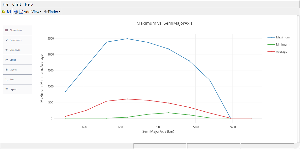
An interesting trend is noted in this study: coverage increases rapidly with altitude until a certain altitude is reached at which point there is an equally sharp drop off. This is due to a resolution constraint of 5 meters – we need to be able to resolve icebergs as small as 5 meters in diameter. Coverage capabilities increase with orbit altitude because the sensor swath also increases. They also decrease beyond a certain altitude because the sensor can no longer resolve 5 meter objects.
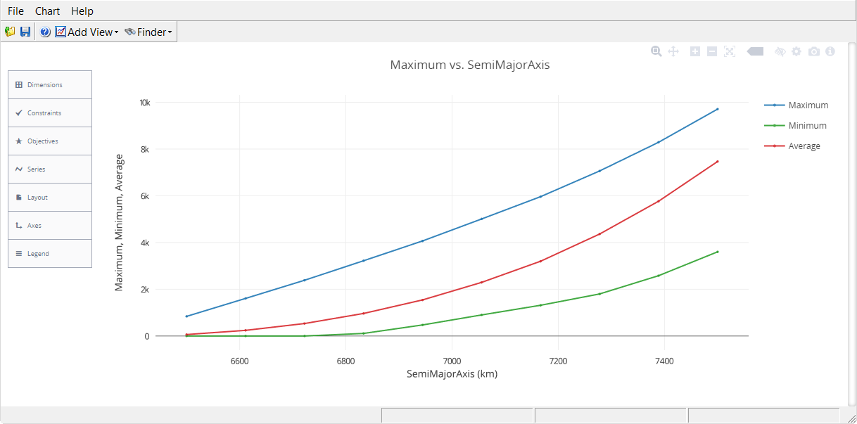
The resulting parametric study indeed indicates that, without a resolution constraint, as altitude increases coverage capabilities also increase.
Our conclusion from this study is that our coverage capability is best with a semi-major axis of about 6,800 km.
Exercise 6. Determine if Inclination and Altitude Impact One Another
We have now determined that inclination and altitude have significant impacts on coverage capability while RAAN has minimal influence. Altitude had an increasingly positive impact until the ground sample distance constraint came into effect. Inclination generally improves as we approach 90 degrees. This leads to two questions:
- Does changing altitude impact our conclusions about inclination?
- Can we improve our sensor characteristics to permit a higher altitude orbit?
We will answer the first question by performing a 2-dimensional parametric study (a.k.a. Carpet Plot). The second question will be answered in later exercises.
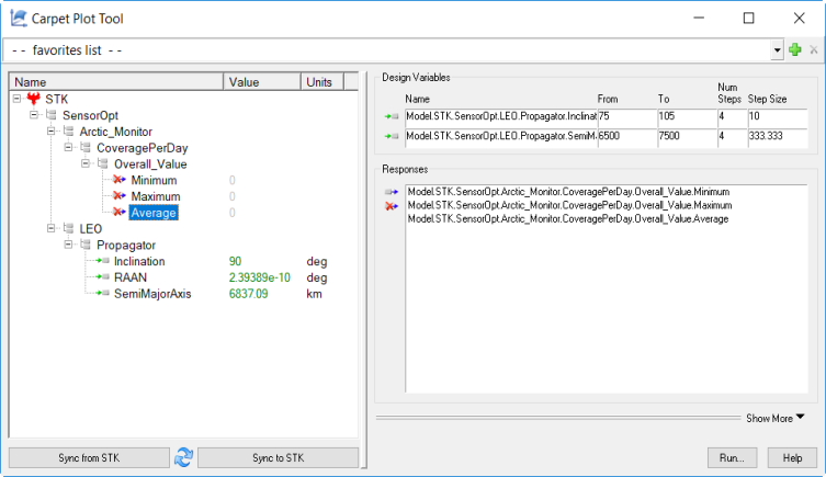
- In the Analyzer window, click on the Carpet Plot icon (
 ) to open a new Carpet Plot study.
 - Fill in the Design Variables (input variables):
- Click Inclination in the Component Tree on the left, and drag it to the input field on the right.
- Set the following values:
- Click SemiMajorAxis in the Component Tree on the left, and drag it to the input field on the right.
- Set the following values:
Option Value starting value: 6500 ending value: 7500 number of samples: 4 step size: 333.333
Option Value starting value: 75 ending value: 105 number of samples: 4 step size: 10 - Fill in the Responses (output variables):
- Click on Minimum in the Component Tree on the left.
- Drag it to the Responses field on the right.
- Repeat the above steps to add Maximum and Average as additional output variables.
-
The Carpet Plot study should look like this:
- Perform the carpet plot by pressing the Run… button. Note that no plots will appear for this study until all data points have been collected.
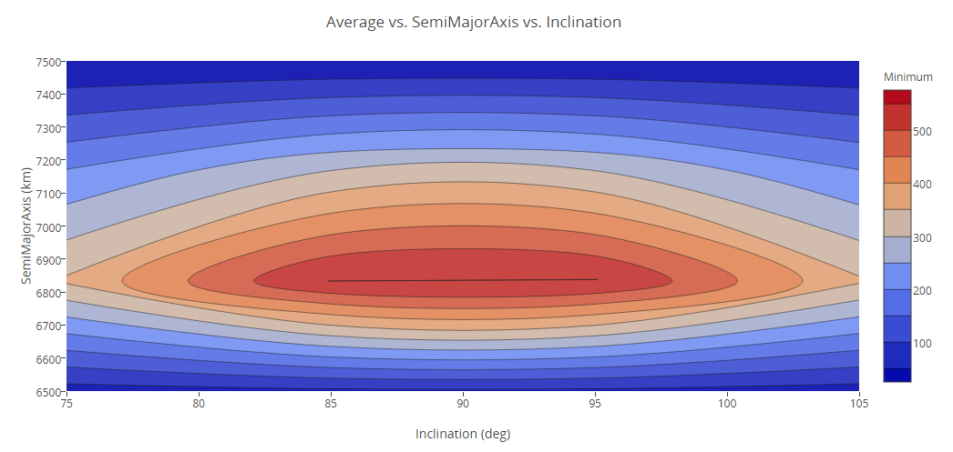
- Create a Contour Plot.
- On the Table - Trade Study window, click the Add View drop down, and select Contour Plot.
- Update the graph to display Inclination vs Semi Major Axis vs Average coverage time.
- In the Contour Plot window, click on Dimensions () in the menu list.
- Click the x drop down box, and select Inclination.
- Click the y drop down box, and select SemiMajorAxis.
- Click the z drop down box, and select Average.
- Select Series () in the menu on the left.
- In the Series drop down at the top, select All series (contour).
- Click on the graph to exit out of the menu.
- In the Contour Plot window, click on Dimensions (
- The Contour plot indicates that, regardless of altitude, the likely optimal inclination is around 90 degrees.
- To examine the data further, add a new plot to be used to display the minimum coverage time.
- Create a 3D Surface Plot.
- On the Contour Plot window, click the Add View drop down, and select Legacy Views...
- On the new Trade Study window that pops up, click the Standard Plots drop down, and select 3D Surface Plot.
- Click Chart on the Menu bar, and select Basic Settings.
- On the Variables tab, ensure:
- design variable 1 (Inclination) is on the X axis
- design variable 2 (SemiMajorAxis) is on the Z axis
- response (Minimum coverage time) is the Y Plot Variable
- Click OK to dismiss the Basic Settings window.
- The resulting graph will now display the minimum coverage time plotted for varying inclination values.
- Create a 3D Surface Plot.

Knowing the inclination is best at 90 degrees, and RAAN is relatively insignificant; our goal now becomes to improve our sensor characteristics to allow for greater orbit altitude and thus improve coverage.
- Close the Carpet Plot Tool window.
Exercise 7. Determine Sensor Impacts on Coverage
We now know that for any given inclination, increasing orbit altitude will improve coverage capabilities until we run up against the ground sampling resolution constraint for the sensor. Fortunately, we can change sensor parameters to permit greater viewing capabilities at higher altitudes.
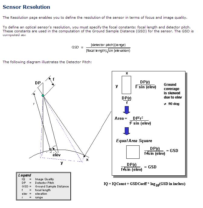
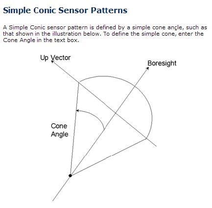
Ground sampling distance, as shown below, is a function of both focal length and detector pitch for a sensor.
This exercise contains the following studies:
- Impact of Detector Pitch on Coverage.
- Impact of Focal Length on Coverage.
- Impact of the Sensor Cone Angle.
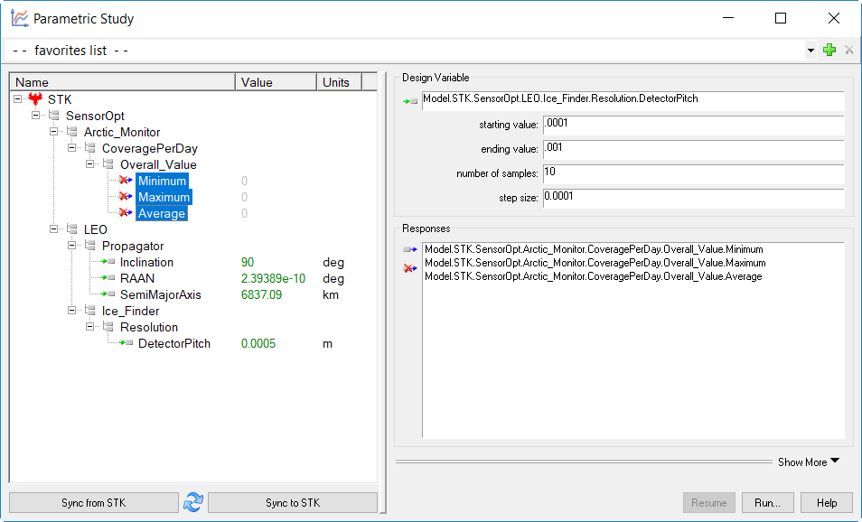
Impact of Detector Pitch on Coverage
This study will show how changing the detector pitch will impact coverage for a variety of altitudes.
- On the Analyzer window, add detector pitch, focal length, and cone angle as input variables.
- In the STK Variables list, select the LEO satellite's Ice_Finder sensor.
- In the STK Property Variables, extend Resolution.
- Click and drag DetectorPitch to the Analyzer Variables section or click select DetectorPitch and move () it to the Analyzer Variables section. It will show up under the Inputs list.
- Repeat the previous step for FocalLength.
- In the STK Property Variables, extend SimpleConic.
- Click and drag coneAngle to the Analyzer Variables section or click select coneAngle and move () it to the Analyzer Variables section. It will show up under the Inputs list.
- Click on the Parametric Study icon () to open a new Parametric Study.
- Fill in the Design Variable (input variable):
- Click DetectorPitch in the Component Tree on the left.
- Drag it to the input field on the right.
- Set the following values:
Option Value starting value: .0001 ending value: .001 number of samples: 10 step size: .0001
- Fill in the Responses (output variables):
- Click on Minimum in the Component Tree on the left.
- Drag it to the Responses field on the right.
- Repeat the above steps to add Maximum and Average as additional output variables.
-
The Parametric Study should look like this:
- Perform the study by pressing the Run… button.
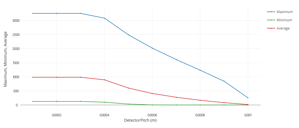
- Update the graph to display DetectorPitch vs the Maximum, Minimum, and Average coverage time.
- In the 2D Scatter Plot window, click on Dimensions () in the menu list.
- Click the x drop down box, and select DetectorPitch.
- Ensure Maximum is selected as the y value.
- Click the plus sign at the top of the Dimensions window to create "Series 2".
- Click the x drop down box, and select DetectorPitch.
- Click the y drop down box, and select Minimum. This will change "Series 2" to "Minimum".
- Click the plus sign at the top of the Dimensions window to create "Series 3".
- Click the x drop down box, and select DetectorPitch.
- Click the y drop down box, and select Average. This will change "Series 3" to "Average".
- Select Series () in the menu on the left.
- In the Series drop down at the top, select All series (scattergl).
- Selectas the line marker.
- Click on the graph to exit out of the menus.
- In the 2D Scatter Plot window, click on Dimensions (
We can conclude from these results that detector pitch has a maximum threshold value (.0003 m), which if exceeded will result in degraded coverage capabilities. Our goal then is to know what this threshold value is for a given orbit and sensor configuration.
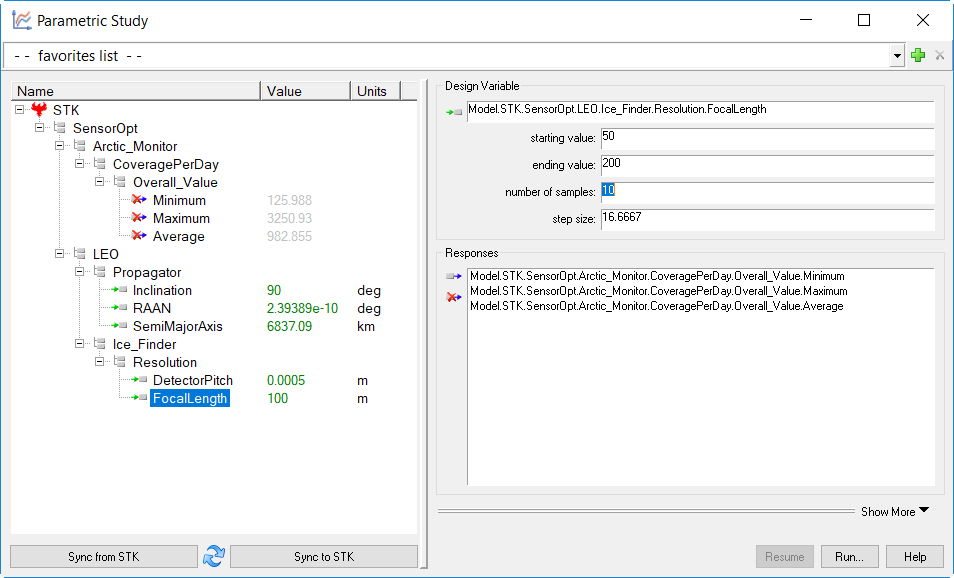
Impact of Focal Length on Coverage
The following study will determine the impacts of focal length on coverage.
- In the Parametric Study window, delete the DetectorPitch from the Design Variable section.
- Fill in the Design Variable (input variable):
- Click FocalLength in the Component Tree on the left.
- Drag it to the input field on the right.
- Set the following values:
Option Value starting value: 50 ending value: 200 number of samples: 10 step size: 16.6667 - The Responses should remain Minimum, Maximum, and Average coverage time.
- The Parametric Study should look like this:
- Perform the study by pressing the Run… button.
- Update the graph to display FocalLength vs the Maximum, Minimum, and Average coverage time.
- In the 2D Scatter Plot window, click on Dimensions () in the menu list.
- Click the x drop down box, and select FocalLength.
- Ensure Maximum is selected as the y value.
- Click the plus sign at the top of the Dimensions window to create "Series 2".
- Click the x drop down box, and select FocalLength.
- Click the y drop down box, and select Minimum. This will change "Series 2" to "Minimum".
- Click the plus sign at the top of the Dimensions window to create "Series 3".
- Click the x drop down box, and select FocalLength.
- Click the y drop down box, and select Average. This will change "Series 3" to "Average".
- Select Series () in the menu on the left.
- In the Series drop down at the top, select All series (scattergl).
- Selectas the line marker.
- Click on the graph to exit out of the menus.
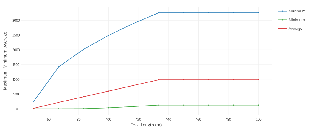 Like detector pitch, focal length also has a threshold value (133.333 m) that when reached, does not improve coverage capabilities.
 - In the 2D Scatter Plot window, click on Dimensions (
Impact of the Sensor Cone Angle Parameter
The following study will determine the impact of the cone angle sensor parameter.
- In the Parametric Study window, delete the FocalLength from the Design Variable section.
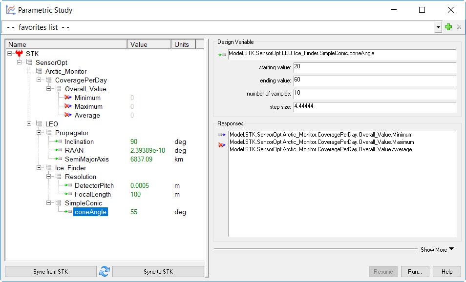
- Fill in the Design Variable (input variable):
- Click coneAngle in the Component Tree on the left.
- Drag it to the input field on the right.
- Set the following values:
Option Value starting value: 20 ending value: 60 number of samples: 10 step size: 4.44444 - The Responses should remain Minimum, Maximum, and Average coverage time.
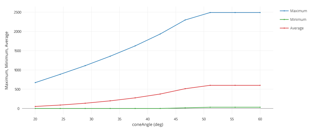
- The Parametric Study should look like this:
- Perform the study by pressing the Run… button.
- Update the graph to display FocalLength vs the Maximum, Minimum, and Average coverage time
- In the 2D Scatter Plot window, click on Dimensions () in the menu list.
- Click the x drop down box, and select coneAngle.
- Ensure Maximum is selected as the y value.
- Click the plus sign at the top of the Dimensions window to create "Series 2".
- Click the x drop down box, and select coneAngle.
- Click the y drop down box, and select Minimum. This will change "Series 2" to "Minimum".
- Click the plus sign at the top of the Dimensions window to create "Series 3".
- Click the x drop down box, and select coneAngle.
- Click the y drop down box, and select Average. This will change "Series 3" to "Average".
- Select Series () in the menu on the left.
- In the Series drop down at the top, select All series (scattergl).
- Selectas the line marker.
- Click on the graph to exit out of the menus.
- In the 2D Scatter Plot window, click on Dimensions (
- Close the Parametric Study window.
The cone angle, like the other parameters also has a threshold value (51 deg).
Exercise 8. Optimize Sensor Parameters
We now know that sensor parameters have a large impact on coverage capabilities. In order to optimize these parameters, we can either guess at values, or employ an optimization tool. Although we can clearly see trends from the previous studies, guessing at values will be difficult because we are dealing with multiple parameters at the same time and the trends we have studied thus far assume only one or two parameters are changed at a time.
To solve more complex problems, an optimization tool can be a very useful guide. An optimizer is an automated tool that makes mathematical calculations about a design problem and incrementally attempts to find an optimal solution. The algorithm we will employ here is the Design Explorer’s SEQOPT algorithm. The SEQOPT intelligently utilizes surrogate models to accelerate the optimization process. The algorithm is used to systematically modify variables in a Scenario until some objective is met.
The optimizer will be used in this problem to minimize the focal length requirement for the sensor while maintaining a minimum coverage capability of 150 seconds per day for our coverage area.
- Select the OptimizationToolButton (
 ) from the
Analyzer toolbar.
) from the
Analyzer toolbar. - Fill in the Optimization Tool:
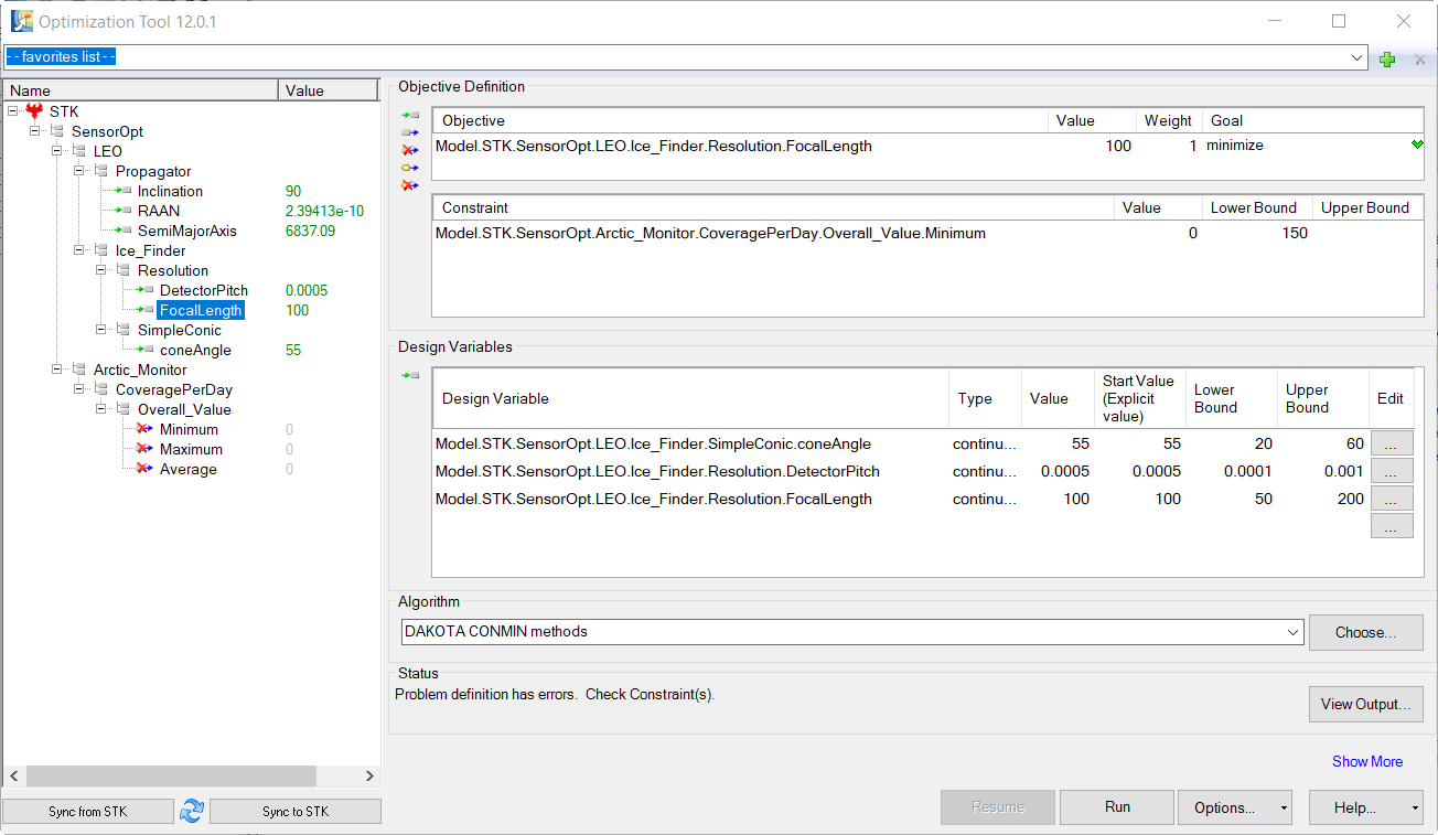
- Select FocalLength in the Components Tree on the left, and drag it to the Objective field on the right.
- The value should be 100, and the Goal is minimize.
- Select Minimum coverage time in the Components Tree on the left, and drag it to the Constraint field on the right.
- Set the Lower Bound to 150.
- Select coneAngle in the Components Tree on the left, and drag it to the Design Variable field on the right.
- Set the lower bound = 20, and upper bound = 60.
- Select DetectorPitch in the Components Tree on the left, and drag it to the Design Variable field on the right.
- Set the lower bound = 0.0001, and the upper bound = 0.001.
- Select FocalLength in the Components Tree on the left, and drag it to the Design Variable field on the right.
- Set the lower bound = 50, and the upper bound = 200.
- Select DAKOTA CONMIN methods in the Algorithm drop down list.
- Make sure that the initial values of the Analyzer variables, marked in green in the variable tree on the left, match the values in the picture below. Take special care that the inclination is equal to 90 degrees. If your values don't match the picture below, click the Sync From STK button. These values are vital to insure your analysis converges to an answer.
The Optimization Tool should look like this:
- Perform the optimization study by pressing the Run… button. The optimizer will display a history of steps as it progresses.
- When the optimization study is complete, click the View Output button on the Optimization Tool window.
- Select the Best Design tab, and view the results.
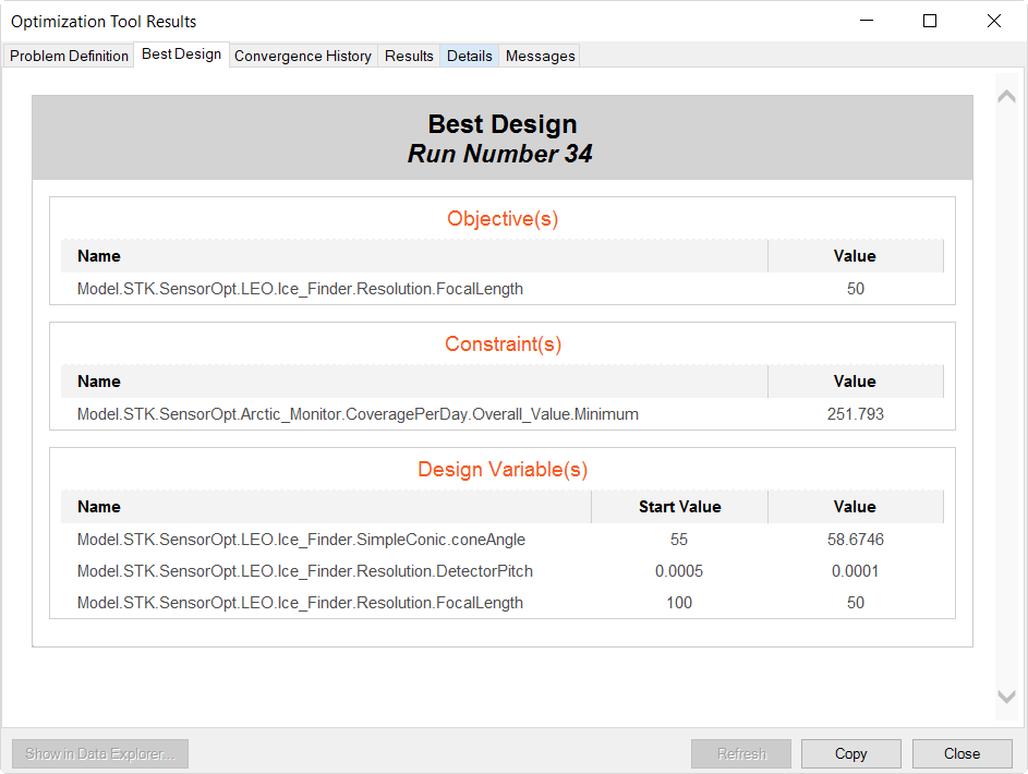
These settings are instructing the optimizer to try and minimize the value for FocalLength by changing coneAngle, DetectorPitch, and FocalLength all while maintaining a minimum coverage value of 150.
The optimizer was able to drive focal length to its lower bound of 50 while at the same time exceeding the goal of 150 minimum seconds of coverage for all grid points.
After running an optimization study, the values in your Scenario will be changed to the final, optimized values. They will not be changed back to what they were before starting the study.
 Visit AGI.com