In this case study, we will describe how angular velocity and acceleration computations are performed in STK in order to explain differences in three attitude files sampled at three different periods (1 second, 10 seconds and 60 seconds).
In general, whenever derivative information is not available, STK resorts to numerical differentiation using central differencing, if possible, or forward/backward differencing at the end points. Note that derivative information may be absent not only because data files simply do not include it, but also because some formulae or custom plugin attitude definitions choose not to supply it (a typical reason in such cases is that analytical derivative is too cumbersome to compute compared to numerical differentiation).
Note also that majority of functional interfaces in STK are designed to provide both the function and its 1st derivative (it is done to accommodate sampling strategies for threshold crossing that are employed in visibility computations).
Of course, these two factors result in 2nd and higher order derivatives (but usually not the 1st order derivatives) computed using numerical differencing.
A special consideration must be given to sampled data. In STK, the function based on sampled data is derived using polynomial interpolation. Various interpolation methods may include a different number of sampled points resulting in polynomials of different degrees. If derivative information at the sampled points is also available, this information can be included in polynomials yielding functions that not only pass through the sampled points but also pass through them with required slopes. When derivative information is not available (which is the case here), the higher order polynomials produce the more differentiable functions; e.g., 1st order polynomials produce continuous but not smooth functions (1st derivatives of such functions are discontinuous) and 2nd order polynomials produce functions that are both continuous and smooth (1st derivatives of such functions are continuous). Note that while higher order polynomials produce smoother functions they are also susceptible to extraneous oscillations or “ringing” which can generate interpolated values that deviate significantly from the sampled points. The best practice is to generate a sufficient number of samples (as generally prescribed by the Nyquist period) and then use a relatively low-order polynomial to interpolate in between.
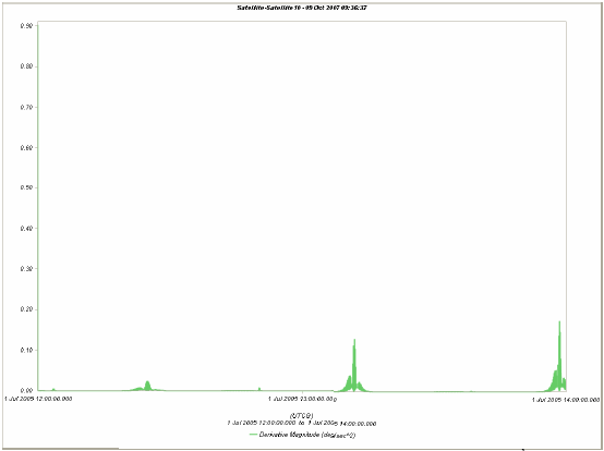
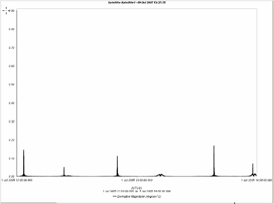
Now we can examine specifics of the case at hand. We have three files with attitude data sampled at three different periods (1 sec, 10 sec and 60 sec). Each file includes only quaternion samples. The default interpolation order for attitude data is 1. When applied to attitude, 1st order interpolation produces a fixed rate eigen-axis slew between any two sampled points. Of course, the rate will change discontinuously when transitioning from one pair of attitude samples to the next. When this data is passed to numerical differencing routine, the angular acceleration ends up being either zero or some finite value depending on how samples used for differencing fall with respect to the samples in the file. In STK, the central differencing of attitude data is set to use points +/-0.1 seconds apart from the time of interest. Since this is smaller than 1 second – the smallest data sampling among the presented three cases, all of them produce angular acceleration that remains at zero most of the time but spikes to some finite value whenever central differencing samples happen to fall on opposite sides of the attitude sample in the file. The size of each spike will depend on the differences in angular velocity values across the discontinuity divided on the differencing interval (0.2 sec for central differencing). See Attitude Data Using 1 Second Samples and 1st Order Attitude Interpolation.
Of course, attempting numerical differencing on discontinuous data is not advisable. There are two possible ways to solve the problem:
- Include sampled angular velocity data in the files and preserve 1st order interpolation. This option is preferable because it will generate more accurate and better behaved interpolated function. In addition to Lagrange, it can support Hermite interpolation, which can prevent aliasing of revolutions and ringing common with sparsely populated cyclical data.
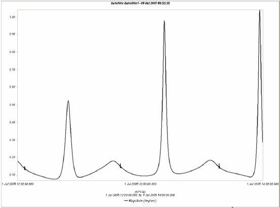
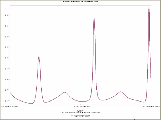
- Interpolate attitude using 2nd or higher orders of interpolation without sampled angular velocity. This option may improve computation of angular acceleration in the absence of angular velocity samples but may also suffer from high sensitivity to sample errors and from Runge’s phenomenon – large departures of the interpolation polynomial from sampled points. This result is illustrated in figures below where linear, quadratic and cubic attitude interpolations are applied to generate angular velocity and angular acceleration plots based on 60 second attitude samples. Note that both quadratic and cubic interpolations produce angular accelerations that change gradually (although still fast at times) and no longer jump between zero and non-zero values, and that cubic interpolation produces smoother angular velocity than quadratic interpolation. At the same time, there are still significant discrepancies in angular acceleration due to interplay between original attitude samples and interpolated samples used for numerical differentiation. In general, higher derivatives of the interpolated data can be obtained analytically by repeated differentiation of the interpolation polynomials.
These two options are controllable using simple keywords in an Attitude file.
Attitude Data Using 1 Second Samples and 1st Order Attitude Interpolation
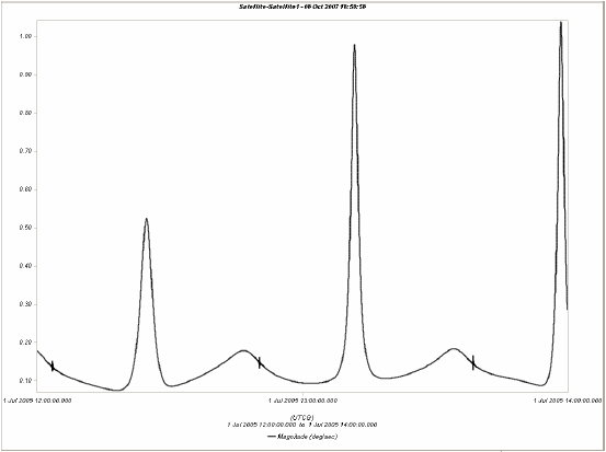
The following shows angular velocity in J2000 using 1 second samples and 1st order attitude interpolation:
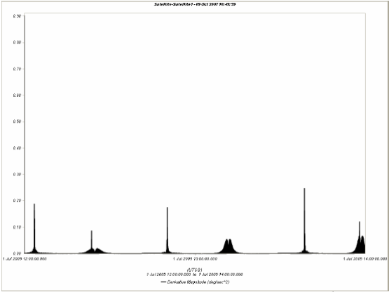
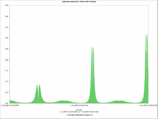
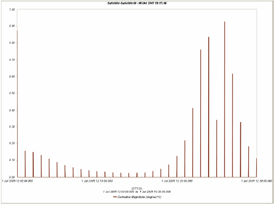
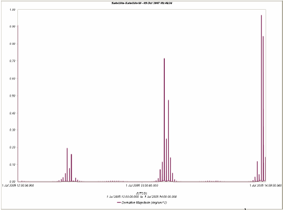
The following shows angular acceleration in J2000 using 1 second samples and 1st order attitude interpolation:
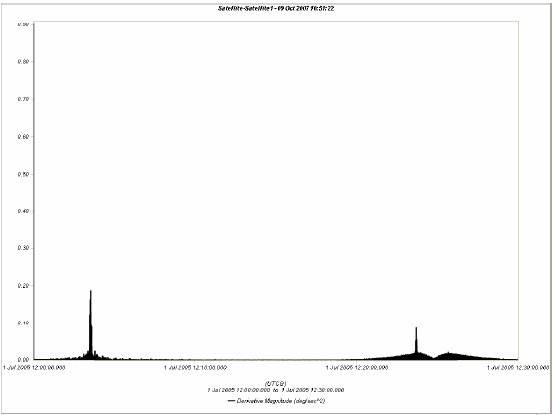
The following shows details of angular acceleration in J2000 using 1 second samples and 1st order attitude interpolation for the first 30 minutes:
Attitude Data Using 10 Second Samples and 1st Order Attitude Interpolation
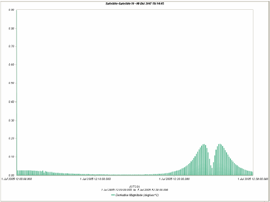
The following shows details of angular acceleration in J2000 using 10 second samples and 1st order attitude interpolation:
The following shows details of angular acceleration in J2000 using 10 sec samples and 1st order attitude interpolation:
The following shows details of angular acceleration in J2000 using 10 second samples and 1st order attitude interpolation for the first 30 minutes.
Attitude Data Using 60 Second Samples and 1st Order Attitude Interpolation
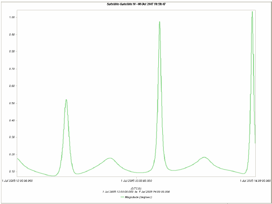
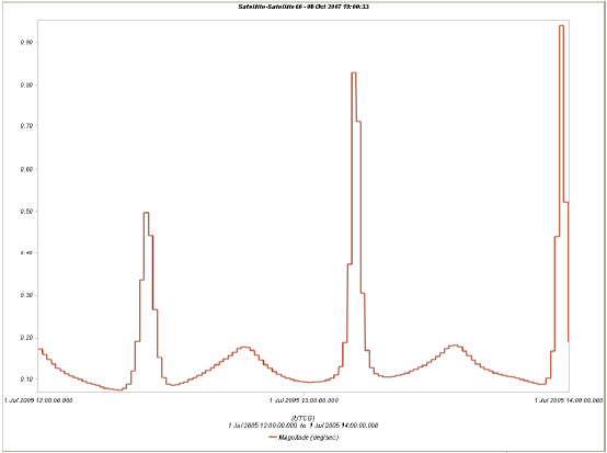
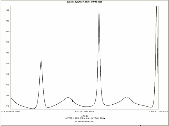
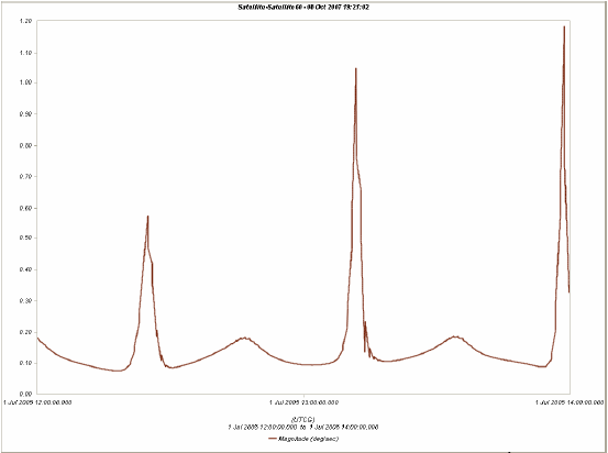
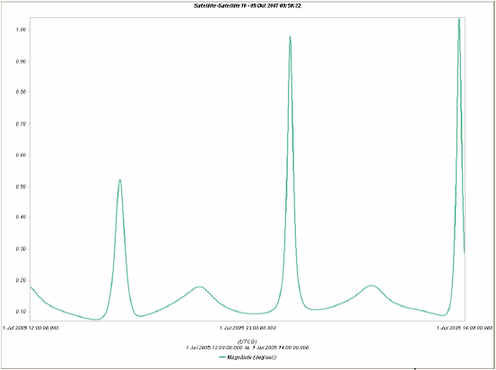
The following shows details of angular velocity in J2000 using 60 second samples and 1st order attitude interpolation:
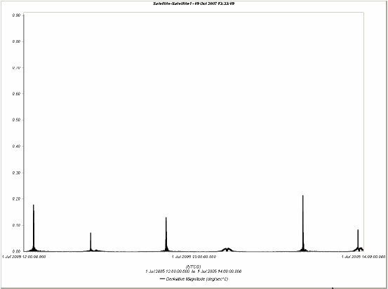
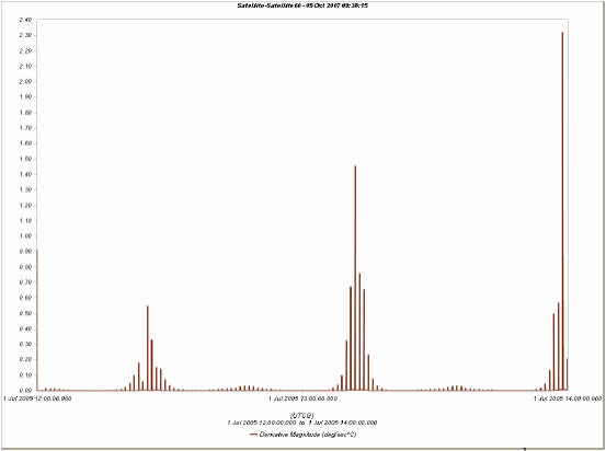
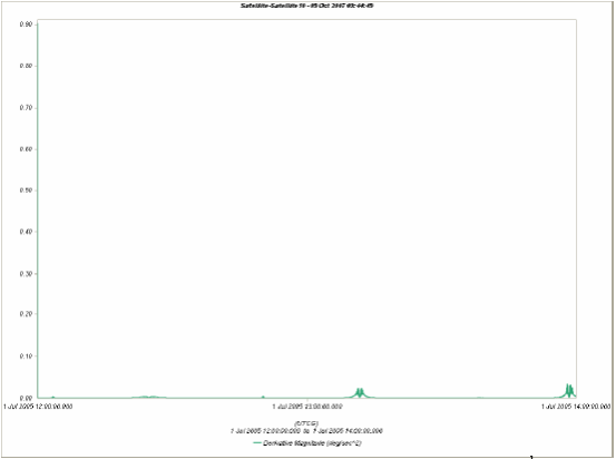
The following shows angular acceleration in J2000 using 60 second samples and 1st order attitude interpolation:
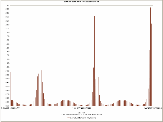
The following shows angular acceleration in J2000 using 60 second samples and 1st order attitude interpolation for the first 30 minutes:
Attitude Data Using 1 Second Samples and 2nd Order Attitude Interpolation
The following shows angular velocity in J2000 using 1 second samples and 2nd order attitude interpolation:
The following shows angular acceleration in J2000 using 1 second samples and 2nd order attitude interpolation:
Attitude Data Using 10 Second Samples and 2nd Order Attitude Interpolation
The following shows angular velocity in J2000 using 10 second samples and 2nd order attitude interpolation:
The following shows angular acceleration in J2000 using 10 second samples and 2nd order attitude interpolation:
Attitude Data Using 60 Second Samples and 2nd Order Attitude Interpolation
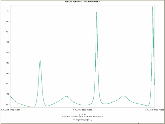
The following shows angular velocity in J2000 using 60 second samples and 2nd order attitude interpolation:
The following shows angular acceleration in J2000 using 60 second samples and 2nd order attitude interpolation:
Attitude Data Using 1 Second Samples and 3rd Order Attitude Interpolation
The following shows angular velocity in J2000 using 1 second samples and 3rd order attitude interpolation:
The following shows angular acceleration in J2000 using 1 second samples and 3rd order attitude interpolation:
Attitude Data Using 10 Second Samples and 3rd Order Attitude Interpolation
The following shows angular velocity in J2000 using 10 second samples and 3rd order attitude interpolation:
The following shows angular acceleration in J2000 using 10 second samples and 3rd order attitude interpolation:
Attitude Data Using 60 Second Samples and 3rd Order Attitude Interpolation
The following shows angular velocity in J2000 using 60 second samples and 3rd order attitude interpolation:
The following shows angular acceleration in J2000 using 60 second samples and 3rd order attitude interpolation:
 Visit AGI.com