Astrogator.
This tutorial will show some basic steps in modeling missions of one satellite approaching another already in orbit using STK Astrogator. In this example, you will model two satellites already in the same plane, with an “Inspector” trailing a “Target Satellite” in True Anomaly, and will target two in-plane burns to approach and subsequently circumnavigate the target. We’ll create an Astrogator Mission Control Sequence to perform a non-optimal transfer to the target satellite, and a maneuver to enter into a Natural Motion Circumnavigation relative orbit.
It is worth noting that there is nothing trivial about Rendezvous and Proximity Operations (RPO). This tutorial is intended to address a common RPO mission requirement, while providing a basic understanding of Astrogator techniques. It is not meant to cover or address all of the nuances regarding this type of relative orbit. As mentioned above, this tutorial will not result in a minimum delta V solution, as osculating orbital effects are not considered in determining optimal departure and transfer times.
Recommended Astrogator Training
This tutorial assumes you have some working knowledge of STK Astrogator. It is recommended you go through the following tutorials to become familiar with Astrogator, if you are not already:
The results of the tutorial may vary depending on the user settings and data enabled (online operations, terrain server, dynamic Earth data, etc.). It is acceptable to have different results.
Watch the following video, then follow the steps below incorporating the systems and missions you work on (sample inputs provided).Model the World!
Before you can begin with any analysis, you need to create a scenario and add a satellite. Let's do that now.
- Create a new scenario and call it Leo_Rendezvous.
- Set the analysis period to the following. Either accept the default start time and add two days (+2 days) or use the specified times below
- Add a satellite (
 ) using the Define Properties (
 ) method in the Insert STK Objects (
 ) tool.
 - Enter the following in the Satellite's properties.
- Change the Initial State (
 ) to the following LEO orbit.
 - Change the Propagation during stopping condition to two (2) days.
| Option | Value |
|---|---|
| Analysis Start Time | 1 Jul 2018 16:00:00.000 UTCG |
| Analysis End Time | + 2 days |
| Option | Value |
|---|---|
| Name | Target_Sat |
| Propagator | Astrogator |
Apopasis Altitude: 500 km
Periapsis Altitude: 500 km
Inclination: 98.5 deg
RAAN: 90 deg
Argument of Perigee: 0 deg
True Anomaly: 0 deg
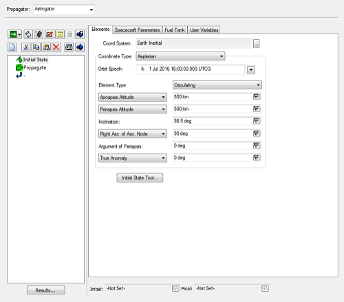
Example LEO orbit values.
Propagate the Satellite and Clean Up Graphics
Now that you have the satellite ready you can propagate it.
- Run (
 ) Astrogator to propagate the satellite.
 - Clear (
 ) the run graphics.
 - Select the 2D Graphics - Pass page.
- Click the Resolution button.
- Set the Maximum time between orbit points to ten (10) sec. This is purely aesthetic.
Create the Inspector Satellite
You have a good start on the inspector satellite with the LEO satellite you just built. Let's copy that satellite and then modify the new copy.
- Copy (
 ) Target_Sat () in the Object Browser.
 - Paste (
 ) the new satellite into the Object Browser.
 - Rename the new satellite RPO_Sat.
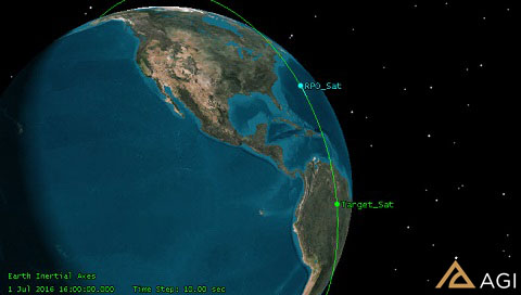
- Open RPO_Sat's properties and on its Basic>Orbit page, modify the True Anomaly to 30 degrees. This will offset RPO_Sat 30 degrees ahead of Target_Sat in an in-plane leading position.
- Change the color of the propagate segment to be a different color than Target_Sat
- Run () Astrogator.
- Clear () the Graphics.
Reference the Target Satellite
- Select the Basic - Reference page in RPO_Sat's () properties ().
- Select Target_Sat as the Reference vehicle.
- Click Select then Apply
This sets the reference for relative parameters, e.g. targeting relative orbit parameters.
Display the RPO Satellite Relative to Target Sat
You can show the RPO trajectory relative to Target_Sat. This is an aesthetic change, but it makes the relative maneuvers easier to understand.
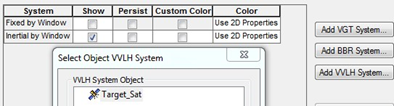
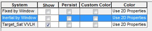
- In the Properties of the RPO_Sat, select the 3D Graphics - Orbit Systems page.
- Click the Add VVLH System button.
- Select Target_Sat and click OK.
- Deselect the other to ensure Target_Sat VVLH is the only one showing.
- Click Apply.
View the RPO Satellite Trajectory
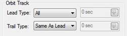
- Select the 3D Graphics - Pass page.
- Set the Orbit Track Lead Type to All.
- Click OK.
Add an RPO Maneuver to Approach the Target Satellite
- Bring RPO_Sat's () properties () to the front.
- Select the Basic - Orbit page.
- Change the existing Propagate (
 ) segment duration to 600 seconds.
 - Add a Target Sequence (
 ) after the propagate segment.
 - Name the new Target Sequence Target Approach.
This propagation time is an arbitrary selection based on an initial guess for a mission requirement, and may not be optimal. For an optimal (minimum Delta V) solution, a Lambert solver can be used to seed an initial guess two-body guess to Astrogator. Conversely, the optimization profiles of SNOPT or IPOPT can be utilized within Astrogator. This will be discussed at the end of the tutorial.
Add an In-Plane Maneuver
First you will do an in-plane maneuver to cause the satellite to drift to a specific point (in RIC coordinates) relative to the target satellite.
- Insert a Maneuver Segment inside the Target Sequence, and name it Burn1.
- In the properties panel for the “Burn1” maneuver, change the Attitude Control option to Thrust Vector.
- Click the ellipses next to thrust axes. Ensure that All STK Objects is selected in the filter dropdown, and select RPO_Sat as the object. Select the RIC axess on the right side as the thrust axes.
- Click the targets beside the X, Y, and Z values. They should become checked (
 ). Keep the default 0 m/s values for each dimension, this serves as the initial guess for the target sequence.
Drift Toward the Satellite
- Add a new propagate () segment after the Maneuver (
 ).
). - Rename the propagate segment Drift.
- Set the Drift Propagate duration trip value to ten (10) hours. This will have an impact on the drift rate: 30 deg drift in 10 hours -> 3 deg/hour.
- Set the color of the Drift propagate segment to something different than the Target_Sat color.
- Run () Astrogator.
This propagation time is an arbitrary selection based on an initial guess for a mission requirement, and my not be optimal. For an optimal (minimum Delta V) solution, a Lambert solver can be used to seed an initial guess two-body guess to Astrogator. Conversely, the optimization profiles of SNOPT or IPOPT can be utilized within Astrogator. This will be discussed at the end of the tutorial.
RPO drifting with Target_Sat
Set Goals for the Target Sequence
You would like to target a desired position relative to Target_Sat at the end of the drift propagate segment. You can specify those desired values and solve for them using the Target Sequence.
- Select the Drift Propagate segment in the Mission Control Sequence (MCS) Browser.
- With Drift selected, click the Results button.
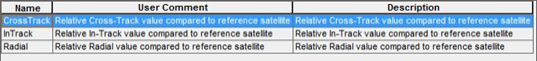
- Expand (
 ) the Relative Motion Components directory.
 - Move (
 ) CrossTrack, InTrack, and Radial to the Selected Components field.
 - Click OK.
Set the Differential Corrector Search Profiles
Rather than attempting to force a single Differential Corrector to solve for the maneuver components in three axes all at once, we’re going to nest multiple differential correctors to quickly “walk into” our solution.
Build First Differential Corrector
- Select the Target Approach target sequence in the MCS.
- By default there will be one Differential Corrector profile in the target sequence’s properties panel. Rename the existing Differential Corrector Target InTrack.
- Open the properties of the “Target InTrack” differential corrector.
- In this first profile, we’re only going to solve for the InTrack maneuver component. For the Y Maneuver component perform the following:
- Enable the Use option.
- Set the Perturbation to 1 m/sec.
- Set the Max Step to 10 m/sec.
- As an equality constraint, we want to achieve a relative InTrack position. For the InTrack result, perform the following:
- Enable the Use option.
- Set the desired value to be 1 km.
- Set the Tolerance to 0.001 km.
- Click the Convergence Tab at the top of the dialog.
- In the Convergence Criteria drop box, select the following:
- Click OK.
- Save your scenario.
Setting the Perturbation and Max Step sizes appropriately for your differential corrector is an important step. If set too large or too small, it can prevent the differential corrector from converging on a solution. It is important to think through the magnitude of the changes required for each control parameter in the differential corrector, and to set these fields accordingly.

Build Second Differential Corrector
- In the target sequence’s properties panel, click the copy button (
 ) to copy the differential corrector. Click the paste button (
  ) to paste a copy.
 - Rename the Copy Target Radial & InTrack.
- Open the properties of the new differential corrector.
- Make sure the Y Maneuver component is still enabled.
- For the X Maneuver component perform the following:
- Enable the Use option.
- Set the Perturbation to 1 m/sec.
- Set the Max Step to 10 m/sec.
- Make sure the InTrack result is still enabled.
- We need to add the relative radial position as an equality constraint. For the Radial result, perform the following:
- Enable the Use option.
- Set the Tolerance to 0.001 km.
- In the Scaling Method drop-down box, choose By Tolerance.
- Click OK.
In this differential corrector, we will use the solution previously determined for the Y maneuver component, while also solving for the Radial or X maneuver component.
Build Third Differential Corrector
- In the target sequence’s properties panel, click the copy button ( ) to copy the differential corrector. Click the paste button ( ) to paste a copy.
- Rename the Copy Target RIC
- Open the properties of the new differential corrector.
- For the X, Y, and Z Maneuver component perform the following:
- Enable the Use option.
- Set the Perturbation to 1 m/sec.
- Set the Max Step to 10 m/sec.
- Make sure the Radial and InTrack results are enabled.
- We need to add the relative cross-track position as an equality constraint. For the CrossTrack result, perform the following:
- Enable the Use option.
- Set the Tolerance to 0.001 km.
- In the Scaling Method drop-down box, choose By Tolerance.
- Click OK.
- Save your scenario.
In this differential corrector, we will use the solution previously determined for the X and Y maneuver components, while also solving for the Cross-Track or Z maneuver component.
Solve for the Control Parameters
- Set the Action to Run Active Profiles. This informs the target sequence to run the profile and solve for the control parameters to meet the desired results.
- Run () Astrogator to solve for the solution. The sequence should converge. If it does not converge, try adjusting the duration of the Drift propagate segment.
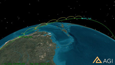
- Right Click on Open the 3D Graphics window and zoom to RPO_Sat. Orient your view so you can see the orbit Astrogator created so far. Notice how RPO_Sat has initiated its transfer to Target_Sat.
- Zoom in on Target_Sat. Notice how the orbital trace for RPO_Sat stops 1km away from it, on the VBar or In-track direction relative to Target_Sat.
Target a Maneuver to Circumnavigate the Target Sequence
We’ve successfully targeted a maneuver to transfer RPO_Sat from it’s initial position 30 degrees away in True Anomaly from Target_Sat, to a position 1km away from Target_Sat on Target_Sat’s VBar. We now need to compute the maneuver required to initiate the relative orbit to circumnavigate Target_Sat in a stable manner.
- Add a 2nd Target Sequence to the end of the MCS. Insert a maneuver segment and it ”Target_NMC.”
You will do a three (3) axis burn to circumnavigate the target. Since you will be starting your circumnavigation relative orbit on Target_Sat’s VBar, it is primarily a radial maneuver required to formulate the orbit. But there are specific conditions that need to be met in order to achieve the natural motion circumnav. The primary condition being that the orbital periods of RPO_Sat and Target_Sat are matched.
- Insert a Maneuver Segment inside the Target Sequence, and name it “Burn2”.
- Change the Attitude Control option to Thrust Vector.
- Click the ellipses next to thrust axes. Ensure that All STK Objects is selected in the filter drop-down, and select RPO_Sat as the object. Select the RIC axes on the right side as the thrust axes.
- Set the X, Y, and Z values to 0.0 m/sec.
- Click the targets beside the X, Y, and Z values. They should become checked (
 ). These values serve as the initial guesses for the target sequence to use for the maneuver components.
Set the Goals of the Target Sequence to Achieve Relative Orbital Parameters
- Select the Burn2 segment in the Mission Control Sequence (MCS) Browser.
- With Burn2 selected, click the Results button.
- Expand () the Formation Components directory.
- Move () Rel Mean SemiMajorAxis to the Selected Components field.
- Expand () the Relative Motion Components directory.
- Move () CrossTrackRate to the Selected Components field.
- Click OK.
Adding this value to the differential corrector will ensure we achieve a relative orbit where the orbital period is matched with Target_Sat’s.
Adding this value to the differential corrector will ensure we achieve a relative orbit that is completely in-plane with Target_Sat.
Add a New Propagate Segment After the Maneuver
- Add a new Propagate () segment after the Maneuver () in the second Target Sequence ().
- Rename the Propagate segment to Prop2PlaneCross.
- Add a new stopping condition of type Y-Z Plane Cross.
- Change the Coordinate System from Earth Inertial by clicking on the ellipses button, selecting Target_Sat in the object list, and then the RIC coordinate system on the right.
- Delete the Duration stopping condition.
- Set the Criterion to Cross Decreasing.
- Click the Results button beneath the MCS for the Prop2PlaneCros segment.
- Open the Relative Motion folder in the component list, and double click InTrack to add it as an equality constraint.
- Change the color of the Propagate segment.
We want Burn2 to generate delta V that will propagate RPO_Sat to the negative VBar or -Y side of Target_Sat. That is essentially a position where RPO_Sat is crossing the YZ Plane of Target_Sat where the YZ plane represents the In-Track/Cross-Track plane of Target_Sat.
We want Burn2 to generate delta V that will propagate RPO_Sat to the negative VBar or -Y side of Target_Sat. That is essentially a position where RPO_Sat is crossing the YZ Plane of Target_Sat where the YZ plane represents the In-Track/Cross-Track plane of Target_Sat in the stopping condition’s properties.
We want to achieve a symmetrical relative position on the negative VBar of Target_Sat from where RPO_Sat is currently. We are currently 1km in the positive VBar. So we want to add a relative position component as the result.
Set the Properties of the Differential Corrector
Similar to the first Target Sequence, we’re going to set up the second Target Sequence to walk into a circumnav relative orbit is a stepwise fashion. To do this, we will use three nested differential correctors.
Build First Differential Corrector
- Select the Target NMC target sequence in the MCS.
- By default there will be one Differential Corrector profile in the target sequence’s properties panel. Rename the existing Differential Corrector Target Radial and InTrack.
- Open the properties of the “Target Radial and InTrack” differential corrector.
- In this first profile, we’re going to solve for the Radial and InTrack maneuver components for the NMC. For the X and Y maneuver components perform the following:
- Enable the Use option.
- Set the Perturbation to 0.1 m/sec.
Ensure the Max Step Size is set to 10 m/sec
- Since we are varying the Radial and InTrack Delta V, we need to add the Relative Semimajor Axis and relative InTrack position as an equality constraints. For the Rel_Mean_Semimajor_Axis result, perform the following:
- Enable the Use option.
- Set the desired value to 0 km.
- Set the Tolerance to 1e-5 km.
- For the InTrack result, perform the following:
- Enable the Use option.
- Set the desired value to -1 km.
- Set the Tolerance to 0.001 km.
- In the Scaling Method drop-down box, choose By Tolerance.
- In the Convergence Criteria drop box, select the following:
- Click OK.
- Save your scenario.
In natural motion relative orbits, the radial and in-track components are intrinsically linked. This can easily be determined by the LTT transformation of the Clohessy-Wiltshire equations. For that reason, it makes sense to solve for the relative radial and in-track components in the same differential corrector.
This will ensure that the maneuver is computed to place RPO_Sat 1km on the other side of Target_Sat when crossing the YZ Plane.
Build Second Differential Corrector
- In the target sequence’s properties panel, click the copy button( ) to copy the differential corrector. Click the paste button ( )to paste the copy.
- Rename the copy Target CrossTrack Rate.
- Open the properties of the new differential corrector.
- Deselect both the X & Y maneuver control parameters.
- In this profile, since we’re only going to solve for the cross-track maneuver component for the NMC, we need to perform the following for the Z maneuver control parameter:
- Enable the Use option.
- Set the Perturbation to 0.1 m/sec.
- Set the Max Step to 10 m/sec.
- Deselect both the Rel_Mean_Semimajor_Axis and InTrack results.
- Since we are varying the cross-track delta V, we need to add the CrossTrackRate as an equality constraint. For the CrossTrackRate result, perform the following:
- Enable the Use option.
- Set the desired value to 0 km/sec.
- Set the Tolerance to 1e-6 km/sec.
- Click OK
- Save your scenario.
In this differential corrector, we will only solve for the cross-track component of the circumnav ellipse. The LTT equations tell us the cross-track component of natural motion ellipses are de-coupled from the radial and in-track components. So solving for it by itself makes sense.
Build Third Differential Corrector
- In the target sequence’s properties panel, click the copy button ( ) to copy the differential corrector. Click the paste button ( ) to paste a copy.
- Rename the Copy Target RI and CrossTrack Rate
- Open the properties of the new differential corrector.
- For the X, Y, and Z Maneuver components perform the following:
- Enable the Use option.
- Ensure the Perturbation is set to 0.1 m/sec.
- Ensure the Max Step is set to 10 m/sec.
- We need to add all three equality constraints. For the Rel_Mean_Semimajor_Axis, InTrack, and CrossTrack results, perform the following:
- Enable the Use option.
- Ensure the CrossTrackRate Tolerance is set to 1e-6km/sec.
- Ensure the Rel_Mean_Semimajor_Axis Tolerance is set to 1e-5km/sec.
- Ensure the InTrack Tolerance is set to 0.001km.
- In the Scaling Method drop-down box, choose By Tolerance.
- Click OK.
- Save your scenario.
In this differential corrector, we will use the solutions previously determined for the X, Y, and Z maneuver components, and further refine them in a single differential corrector.
Propagate the Natural Motion Circumnav for 12 Hours
- After the Target NMC target sequence, add a propagate segment and name it NMC.
- Set the trip value for the duration stopping condition to be 12 hours.
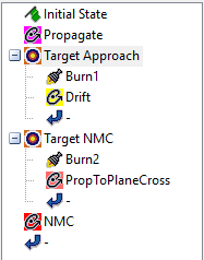
- Your MCS should look like this:
Solve for the Control Parameters
- For the Target NMC target sequence, set the Action to Run Active Profiles. This informs the target sequence to run the profile and solve for the control parameters to meet the desired results.
- Run () Astrogator to solve for the solution.
- Clear () the graphics.
![]()
Evaluate the Maneuvers Performed
Take a look at the differential correct window for the second target sequence (Target NMC) where we targeted the Radial, InTrack, and CrossTrack Rate (Target.NMC.Target RI & CrossTrackRate). It will show you the Delta V magnitude for each maneuver axis of the satellite.
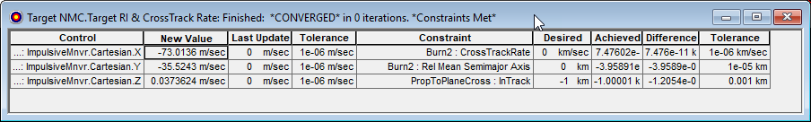
At first glance, the large In-track (Y) maneuver component makes sense. We arrived on Target_Sat’s VBar, and needed to perform an in-track maneuver to move to the negative VBar. What may not make sense is the larger radial (X) maneuver component. What is the reason for this?
Let’s generate a Maneuver Summary report to get a feel for the total delta V required for this maneuver. You can do this two ways.
- Right-click Burn2 in the MCS.
- Select Summary... You can also click the Summary (
 ) button.
 - You can also right-click on RPO_Sat in the Object Browser.
- Select the Report & Graph Manager (
 ).
). - Expand () the Installed Styles directory.
- Generate a Maneuver Summary report.
Notice the delta V magnitude reported:

Take a moment to evaluate the total delta V reported. 81.195 m/sec for Burn2.
Remember that the resulting magnitude of the maneuver vector is computed using the root of the sum of the squares (RSS). So.

It’s worth asking again “why is the radial maneuver required?” What if there was little or no radial component in the maneuver?

The tiny cross-track component wouldn’t even register, and you’d be left with just the expected in-track component.
To understand the reason for the radial component, you need to go back to Burn1, the rendezvous maneuver.
Look at the differential corrector results for the first target sequence (Target Approach).
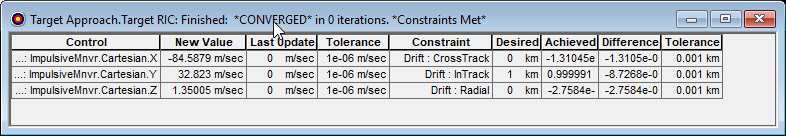
Notice it too has a large radial component of -84.588 m/sec required to perform the maneuver. Remember, RPO_Sat had the same orbital parameters as Target_Sat, but was offset in True Anomaly by 30 degs. In many ways, we would say RPO_Sat was “coplanar” with Target_Sat, with matched inclinations and the same altitude. So why the radial component required?
It goes back to the caveat at the beginning of this lesson. This rendezvous was not optimal.
Effects of Osculating Elements and HPOP
Both Target_Sat and RPO_Sat were propagated in Astrogator using the High Precision Orbit Propagator (HPOP) using osculating elements. What are osculating elements? “Osculating elements are the true time-varying orbital elements, and they include all periodic (long- and short- periodic) and secular effects. They represent the high-precision trajectory and are useful for highly accurate simulations” (Vallado 616; 9.2).
“Osculating elements are the true time-varying orbital elements, and they include all periodic (long- and short- periodic) and secular effects. They represent the high-precision trajectory and are useful for highly accurate simulations” (Vallado 616; 9.2).
If the satellites had been propagated using a two-body propagator, without osculating elements, the cross-track component would dissapear. It just would not have been realistic.
For computing and planning rendezvous using full-force models and osculating elements, choosing optimal departure and arrival times to minimize the differences in orbital periods and other elements is critical. Careful consideration of those time could have minimized the need for much of the radial maneuver component during the rendezvous, and ultimately to maintain the in-track NMC.
Visualize the Osculating Elements
Create an RIC Plot for Target_Sat and RPO_Sat:
- In the object browser, right click on Target_Sat and select Report and Graph Manager.
- Expand the Installed Styles on the right side, and locate and double-click the RIC graph style.
- In the dialog that pops up, select RPO_Sat and click assign.
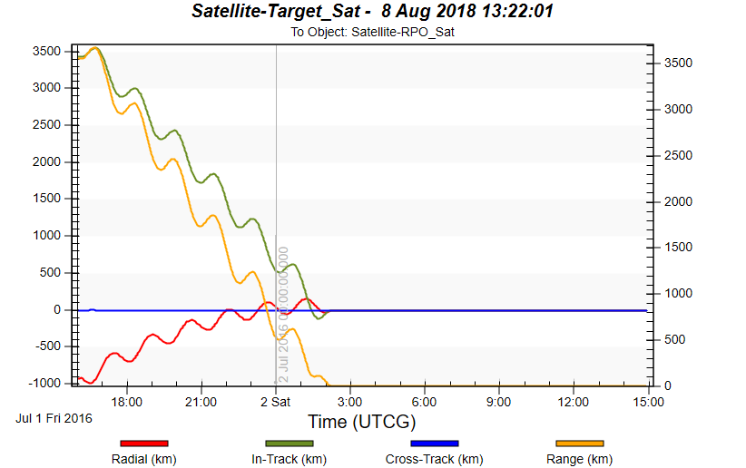
Here we see the RIC plot for Target_Sat to RPO_Sat. It clearly shows the point in time when the rendezvous maneuver takes place, the transfer to RPO_Sat, and when RPO_Sat begins its proximity operations (where the RIC plots converge. Range is drawn on the secondary Y axis.
- Select the zoom tool, and lasso the cross-range plot line from the beginning of the graph to the point when the rendezvous happens.
- Keep zooming in in this manner until you can see the initial maneuver (Burn1) effect the cross-track component.
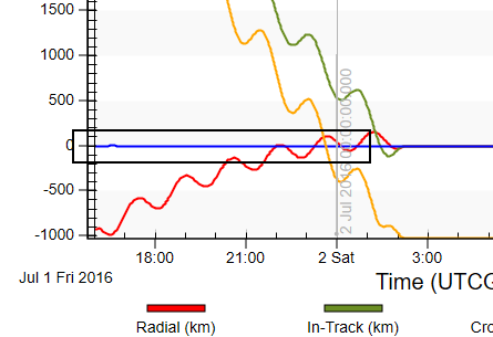
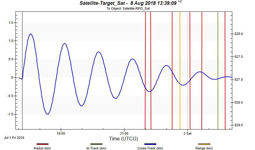
Notice the initial drift in cross-track during the 600sec propagation segment, then the large oscillation that takes place when Burn1 occurs (vertical black line).
The maneuver took place when the relative difference in the cross-track components of Target_Sat and RPO_Sat were not zero. Additionally, we can see that the cross-track component moved by over a kilometer when we initiated the transfer. We needed to raise RPO_Sat’s orbit to drift over to Target_Sat, and it turns out that the rate at which Inclination and RAAN vary, are very sensitive to altitude. So during the transfer, the planes of the two satellites were moving differently and at different rates.
Additionally, to minimize the radial components of the maneuvers and the overall delta V required, careful consideration of the timing of the maneuvers needed to be applied. This can partly be visualized by plotting an altitude plot of RPO_Sat.
Generate an Altitude Plot
- Right-click on RPO_Sat () in the Object Browser and select Report & Graph Manager (
 ).
). - Create a new graph style (
 ), and name it Altitude.
 - Expand (
 ) the Astrogator Values>Geodetic Folder and double click the Altitude data provider.
 - Click OK.
- Click Generate.
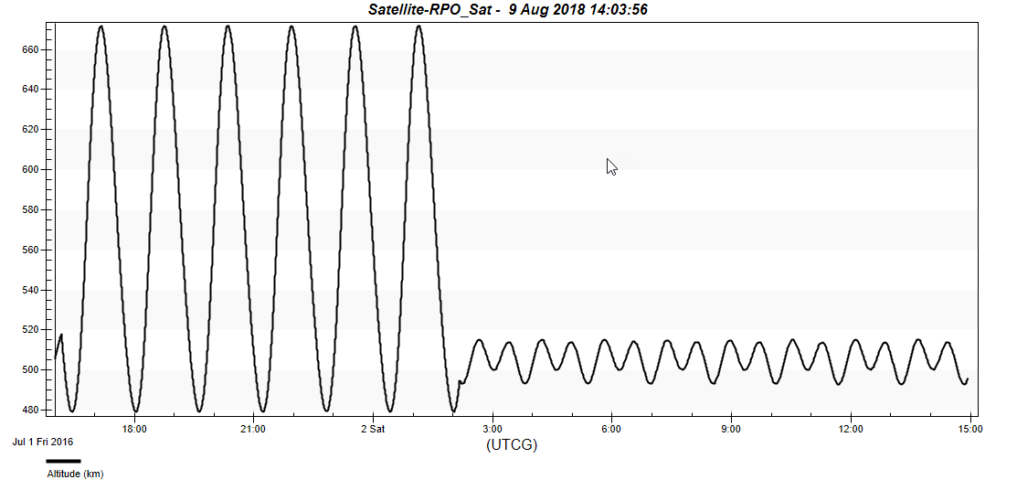
Notice the drastic change in altitude early in RPO_Sat’s ephemeris when it enters the transfer to Target_Sat. Also notice the how there is a jog in the altitude as RPO_Sat enters the NMC around Target_Sat.
These redirections manifest as radial components, and are indicative of sub-optimal departure and arrival times.
A more robust solution incorporating an optimization target profile like IPOPT or SNOPT, to determine the optimal times to initiate the transfer and the drift duration can be implemented.
Enter Near-Optimal Departure and Drift Times
To demonstrate the effect of more-optimal departure and arrival times, enter the following propagations times and re-run the MCS.
- For the initial propagate segment, enter 0 sec for the trip time.
- For the Drift propagate segment, enter 34325 sec for the trip time.
- Re-run the MCS.
How does the total Delta V required compare?
Lastly, a further step of incorporating a minimum delta V Lambert solution into Astrogator via the scripting interface to seed an optimal two-body transfer solution, will greatly increase the efficiency of the transfer and proximity operations maneuvers. Though not necessary, this “semi-analytic” approach of combining analytic solutions from Lambert with the numerical solutions of Astrogator’s search profiles, can be quite successful.
To better understand how our engineers calculated these durations or to use Astrogrator’s built in optimizers to find optimal RPO orbits, try out the follow-on tutorial “Optimal LEO Rendezvous and Proximity Operations.”