STK Pro, STK Premium (Air), STK Premium (Space), or STK Enterprise
You can obtain the necessary licenses for this training by contacting AGI Support at support@agi.com or 1-800-924-7244.
The results of the tutorial may vary depending on the user settings and data enabled (online operations, terrain server, dynamic Earth data, etc.). It is acceptable to have different results.
Capabilities Covered
This lesson covers the following STK Capabilities:
- STK Pro
- Coverage
Problem Statement
The FAA is testing a new experimental radar system which is designed to provide highly accurate location of aircraft as they fly through United States airspace. In order to test the quality of this new system, you will be making a test flight from which you will be monitoring your aircraft's location via GPS. The GPS determined location information will be compared to the radar tracking information to determine the fidelity of the new radar system. In order to accurately test the radar system, you need to know how accurate you can expect the GPS position information to be over the aircraft route.
Break It Down
You have some information that may be helpful. Here’s what you know:
- A positional navigational accuracy (PACC) value of less than ten (10) meters will yield results good enough to use as a reference for your radar.
- You must measure GPS navigational accuracy over the continental United States at the altitude of your flight.
- You must also measure the GPS dilution of precision over the path of a test flight, which will fly from Long Beach to Philadelphia at an altitude of 20,000 feet.
Solution
Using STK's Coverage capability, you will build a scenario to examine navigation accuracy over a large area (the entire airspace of the continental United States). You will determine if there are any areas at any times which would provide an unacceptable navigational accuracy value. If so, you would not be able to use your GPS-reported position to provide a meaningful baseline for a comparison of the radar system's tracking data. Then, you will examine the navigational accuracy values for a specific aircraft route.
Video Guidance
Watch the following video. Then follow the steps below, which incorporate the systems and missions you work on (sample inputs provided).
Create a Scenario
First, you need to define the times during which the conditions that you set for your world, and the objects in your world, will be relevant. Since you are not concerned with examining the navigational accuracy over US airspace on a specific day at a specific time, but instead just doing some general analysis, you can accept the STK default twenty-four (24) hour time period for this example.
-
Click the Create a Scenario (
 ) button.
 - Enter the following in the New Scenario Wizard:
- When you finish, click .
- When the scenario loads, click Save (
 ). A folder with the same name as your scenario is created for you in the location specified above.
 - Verify the scenario name and location and click .
| Option | Value |
|---|---|
| Name | Navigation |
| Description | How will I determine the accuracy of my in-flight navigation solution? |
| Location | C:\Users\<username>\Documents\STK 12\ |
| Start | Leave the default start time. |
| Stop | Leave the default stop time. |
Clean Up
Before you begin to visually define your analysis area, let’s remove all the stuff that you don’t want cluttering up the 2D Graphics window.
- Open the 2D Graphics window properties (
 ).
). - Select the Imagery page.
- Clear the Background Image - Show check box.
- Click to apply the changes and dismiss the Properties Browser.
2D View: 2D Map with only borders and outlines
Define the Analysis Area
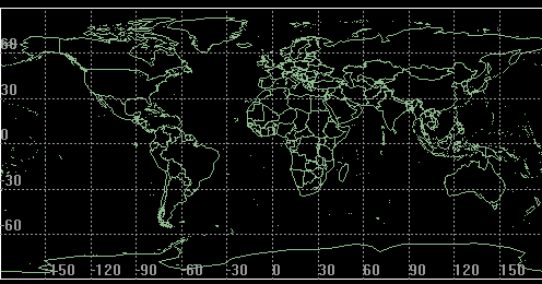
Let's outline the United States on the map so that you can more easily identify and focus on that area of the map.
- Insert an Area Target (
 ) object using the Select Countries And US States (
 ) method.
 - In the Select Countries And US States window, select United_States_of_America.
- Ensure the Primary Area Only option is selected.
- Click .
- Click to dismiss the area target introduction dialog.
Selecting Primary Areas Only during the creation process will ensure that only the continental US is included. If you had selected All Areas, an area target representing each one of the Hawaiian islands, Alaska, etc. would have been imported.
Get a Better Look
- Bring the 2D Graphics window to the front.
- Zoom In (
 ) around the continental United States ().
The United States should now be clearly outlined in the 2D and 3D Graphics windows.
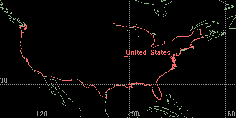
2D View: Area target of the continental US
Remove the Area Target Label
You don’t really need to label the area target or mark the center point of the continental United States for your analysis. Let’s remove the area target marker from United_States_of_America.
- Open United_States_of_America’s () properties ().
- Select the 2D Graphics - Attributes page.
- Set the following:
- Click .
| Option | Value |
|---|---|
| Inherit From Scenario | Off |
| Show Label | Off |
| Show Centroid | Off |
Model Ground Locations
Take a look back at the list you made in the Break It Down section. According to what you know you need to model two locations--the origination and destination locations of your aircraft.
See if you can find a database entry for Philadelphia and Long Beach, and use them to model STK place objects representing the city from which your aircraft will depart (Long Beach) and the aircraft's destination location (Philadelphia).
- Insert a Place (
 ) object using the From City Database (
 ) method.
 - Use the City database to insert the following cities:
- Long Beach, California
- Philadelphia, Pennsylvania
- When you finish, close the City Database Search tool.
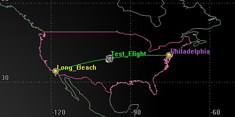
Your departure and destination locations should now be clearly visible on the map in the 2D Graphics window.
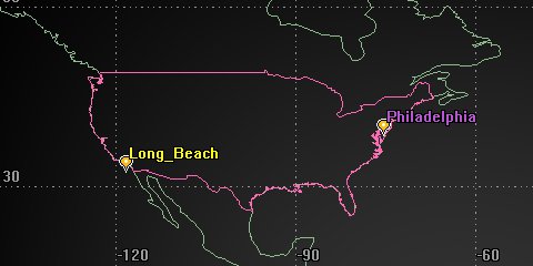
2D View: Philadelphia and Long Beach on the map
Change Your Perspective
How’s that look in 3D?
- Bring the 3D Graphics window to the front.
- Right-click the United_States_of_America () area target.
- Select Zoom To to reposition the view so that United_States_of_America () is the focal point in the 3D Graphics window.
- Use your mouse to zoom out until you can see the entire continental United States.
When you set an area target as the focal point in the 3D Graphics window, STK sets the centroid of the area target as the focal point. You will have to zoom out to see the entire area target.
Using Streaming Terrain for Visualization
By default, streaming terrain is now active in the Globe Manager and visible on the globe if you have an internet connection. If this is the case, make the following changes:
- Open the 3D Graphics window Properties ().
- Select the Details page.
- Select the Enable check box in the Label Declutter section.
- Click .
- Open Navigation's () properties ().
- Select the 3D Graphics - Global Attributes page.
- In the Surface Lines - On Terrain field, select When Terrain Server is on.
- Click .
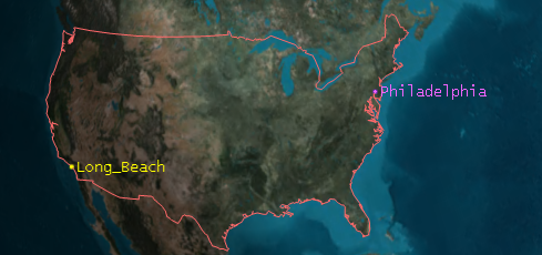
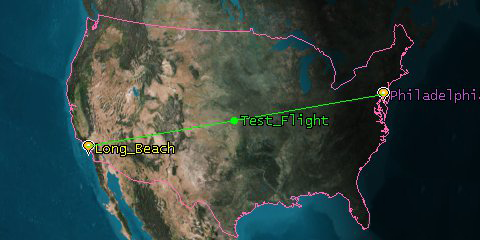
3D View: Philadelphia and Long Beach on the globe
Now, both of your visualization windows are focused on your defined region-of-interest.
Model an Aircraft
You are flying across the continental United States. Your flight takes off from Long Beach and flies to Philadelphia. You have modeled these two cities and now you can model your aircraft and its route.
- Insert an Aircraft (
 ) object using the Insert Default () method.
 - Rename it Test_Flight.
Define Test Flight’s Route
Now you can model Test_Flight’s flight from Long Beach to Philadelphia.
- Bring the 2D Graphics window to the front.
- Open Test_Flight's () properties ().
- With the Basic - Route page open, return to the 2D Graphics window and
- Orient the Properties Browser and the 2D Graphics window so you can see both at the same time.
- Click Long Beach on the 2D Graphics window.
- Return to Test_Flight's () properties ().
- Set the Altitude to 20000 ft.
- Click Philadelphia on the 2D Graphics window.
- Click .
Be careful! Each click on the 2D Graphics window is recognized and added as an aircraft route waypoint.
Get a Better Look
- Position the 2D and 3D Graphics windows so that you can clearly see them both.
- Reset (
 ) the animation.
 - Play (
 ) the animation.
 - Reset () the animation when done.
You can watch Test_Flight fly its route equally well in either 2D or 3D.
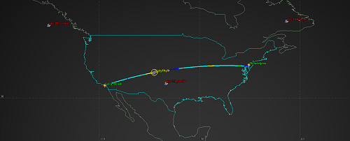
2D View: Test Flight’s route
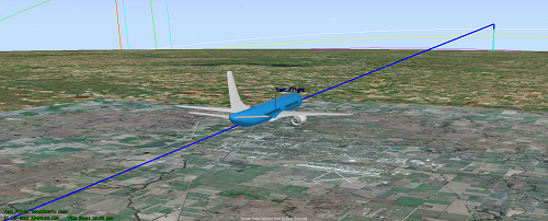
3D View: Test Flight’s route
Model the GPS Network
You also need to model the GPS satellite constellation.
- Insert a Satellite (
 ) object using the Load GPS Constellation (
 ) method.
 - Bring the 3D Graphics window to the front.
- Click the Home View button (
 ) on the 3D Graphics toolbar to restore the default Earth-centered view.
 - Use the mouse to zoom out until you can see the satellites orbit around the globe.
If you do not have an internet connection, you can download the current TLE file. Open the Scenario's Properties and select the Basic - Database page. Or you can download it from AGI's website. You can then insert the GPS database using the From TLE File method.
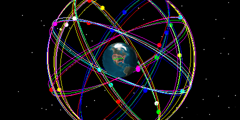
3D View: GPS satellite orbital tracks
By default, the GPSConstellation Orbit tracks are disabled.
How Will I Measure Navigation Accuracy?
You need to assess the accuracy with which you will be able to determine your current position while en route from Long Beach to Philadelphia. You want to assess coverage, or your ability to “see”, over the appropriate number of defined assets throughout the duration of Test_Flight’s flight.
To do this you will assess coverage of the continental United States based on the boundaries of the area target that is being used to outline that area. You will need to specify the region being examined (United_States_of_America), how each grid point should be treated, and what assets will be used to examine the region (GPSConstellation).
Coverage Definition
The first thing you need to do is define the coverage area. Instead of entering the latitude and longitude bounds of the coverage region, you can have STK use the boundaries of your area target to define the boundaries of the coverage definition. Let’s do that now.
- Insert a Coverage Definition object (
 ) using the Insert Default method.
 - Rename the Coverage Definition object ContUS_Cov.
- Open ContUS_Cov's () properties (). The Basic - Grid page displays.
- Change the Grid Area of Interest - Type to Custom Regions.
- Click the button.
- Select United_States_of_America in the Area Targets list.
- Move (
 ) United_States_of_America to the Selected Regions list.
 - Click to return to the Grid page.
- Change the Point Granularity field to Lat/Lon and 1 deg.
- Click to accept the changes and keep the Properties Browser open.
If the Coverage Definition object does not appear in the Insert Objects tool, click the Edit Preferences... button and add it. You can also add the Figure of Merit object since we will use that too.
Get a Better Look
- Bring the 2D and/or 3D Graphics window to the front.
- Answer the following question:
- Is the coverage grid limited to the boundaries of the United States area target?
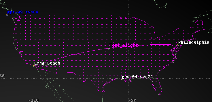
2D View: Coverage grid over continental United States
Define the Altitude of the Grid Points
For your analysis, you want to assess the quality of the navigation solution for an airborne vehicle (Test_Flight) within the continental United States. That means the points to which you want to calculate access will not be on the surface of the Earth. Currently, the coverage grid is on the surface of the Earth. How will you compute coverage to grid points at the same altitude as Test_Flight?
You can associate the properties and constraints of an airborne vehicle, such as Test_Flight, with points in the grid just as you would if you wanted to associate the properties and impose the constraints of a ground-based object, such as a facility, to points on the surface of the Earth. You can associate Test_Flight with the coverage grid, and have points in the grid defined according to Test_Flight’s altitude.
The altitude entered is the altitude used for the coverage definition grid points, not the altitude of the template object. Using a template object would apply any constraints or properties, excluding positional information to each grid point. Since Test_Flight does not have any constraints, we do not need to use this option.
- Return to ContUS_Cov's () properties ().
- In the Point Altitude section, select Altitude Above WGS84 from the drop down.
- Set the Altitude to 20000 ft.
- Click to apply the changes.
- Select the 3D Graphics - Attributes page.
- In the Fill Options section, select the Show at Altitude check box.
- Click to apply changes and keep the Properties Browser open.
Assign Assets
The GPS satellites are the assets with which you want to assess the quality of your coverage. Let’s assign them now.
- Select the Basic - Assets page.
- In the Assets field, select the GPSConstellation (
 ) constellation.
 - Click .
- Click to accept the changes and keep the Properties Browser open.
Don’t Calculate Access ‘Til I Say
In an effort to manage your resources more efficiently, let’s not tie up STK recomputing access automatically every time you make a change. Let’s turn that off. We’ll tell STK when to compute accesses.
- Select the Basic - Advanced page.
- Clear the Automatically Recompute Accesses check box.
- Click to accept the changes and keep the Properties Browser open.
Compute Coverage!
Now that the coverage definition object is defined, you can compute access to points in the grid. Let’s do that now.
- Bring the 2D Graphics window to the front.
- Right-click ContUS_Cov () in the Object Browser.
- Select the Coverage Definition menu.
- Click Compute Accesses.
- When the coverage computations complete, return to ContUS_Cov's () properties ().
- Select the 2D Graphics - Attributes page.
- Clear the Show Points check box.
- Click .
For larger scale calculations, consider computing the accesses for coverage in parallel using multiprocessing. This can be done using multiple cores on a local machine, or taking advantage of cluster configurations, depending upon your machine configuration. For more information on machine configuration, installation of the Parallel Extension, licensing, and more, please see the STK Parallel Cluster Overview.
You can watch the status of the calculations in the Status Bar in the bottom right of the STK GUI.
Navigation Accuracy
Navigation Accuracy measures the uncertainty of a navigation solution based on one-way measurements from a set of transmitters. Most often, the transmitters are those on-board Global Positioning Systems (GPS) satellites. If four or more of these satellites are in view of a ground receiver, a navigation solution consisting of the position of the receiver and the offset between the receiver clock and the GPS clock can be computed.
The Navigation Figure of Merit considers the effect of the number of measurements (of those satellites visible at each moment in time), the geometry of the transmitters and the uncertainty in the one-way range measurements may be specified as a constant value or as a function of the elevation angle on a transmitter basis.
When using Navigation Accuracy to measure the quality of coverage, you need to specify the following settings on the FOM Basic - Definition page:
- Method: Navigation Accuracy to be measured
- Type: Maximum number of assets that can be used to produce navigation solutions
- Compute: Method for computing the static value of Navigation Accuracy over the entire coverage interval.
- Time Step: Step to be used when computing the static value of Navigation Accuracy across the coverage interval
- : Method for computing the range uncertainty for each Coverage asset
Figures of Merit can exhibit two types of behavior: dynamic and static. The dynamic definition of Navigation Accuracy is specified through items 1, 2, and 5, and computes the corresponding value for each grid point at the current time. The static definition of dilution of precision is specified through items 3, 4, and 5, and is computed via sampling of the dynamic definition. While it is important to mention both, in this exercise we will employ the dynamic behavior to show changing PACC graphics for the coast-to-coast aircraft flight.
Method
Navigation Accuracy can be calculated in a number of ways, depending on your task. The methods available to you are discussed in the following table.
| Method | Description |
|---|---|
| GACC (Geometric Accuracy) | Measures the accuracy of the entire navigation solution. GACC combines the accuracy of the position and clock-related components of the navigation solution. |
| PACC/PACC (3) (Position Accuracy) | Measures only the accuracy associated with the positional portion of the navigation solution. |
| HACC/HACC (3) (Horizontal Accuracy) | Measures the accuracy for the horizontal (latitude/longitude) components of the positional portion of the navigation solution. |
| VACC/VACC (3) (Vertical Accuracy) | Measures the accuracy for the vertical (altitude) components of the positional portion of the navigation solution. |
| EACC/EACC (3)* (East Accuracy) | Measures the accuracy in the Eastern component of the positional portion of the navigation solution. |
| NACC/NACC (3)* (North Accuracy) | Measures the accuracy in the Northern component of the positional portion of the navigation solution. |
| TACC (Time Accuracy) | Measures the accuracy of the time portion of the navigation solution. |
*If PACC(3), HACC(3), or VACC(3) is selected, the accuracy value is computed even if only three (3) navigation sources are available. This is done by ignoring the clock component of the navigation solution. If four (4) or more sources are available, the clock component is included.
The accuracy measure you choose affects the dynamic and static definition of the figure of merit.
Type
Although four satellites are needed for the navigation solution, additional satellites can be used to improve the accuracy of the solution. Options in the Type field are discussed in the following table.
| Option | Value |
|---|---|
| Over Determined | Computes the NavAcc based on all of the currently available assets. If you select this method, you need to involve a minimum of three assets in the navigation solution. If you compute a navigation accuracy based on only three assets, you will be presented with answers to a subset of main options: PACC, HACC, and VACC. Also, note that a navigation accuracy with three assets assumes no uncertainty in time. |
| Best Four | Computes the NavAcc based on the set of four satellites that yields the minimum GACC. |
| Best N | Computes the NavAcc based on the specified number of satellites that yields the minimum GACC. If you select this method, you also need to specify a value for Best N. |
| Best Four Acc | Computes the NavAcc based on the set of four satellites that yields the minimum geometric uncertainty. |
| Best N Acc | Computes the NavAcc based on the set of the specified number of satellites that yields the minimum geometric uncertainty. If you select this method, you also need to specify a value for Best N. |
The asset selection strategy you choose affects the dynamic and static definition of the figure of merit.
Compute
You also need to set the method for computing the static definition for navigation accuracy using the options in the Compute field. Options are discussed in the following table.
The reported values depend on the specific number selected and the allowed number of assets.
| Option | Value |
|---|---|
| Minimum | Minimum uncertainty at each point over the entire coverage interval |
| Maximum | Maximum uncertainty at each point over the entire coverage interval |
| Average | Computes the NavAcc based on the specified number of satellites that yields the minimum GACC. If you select this method, you also need to specify a value for Best N. |
| % Below | The value of the uncertainty is less than the computed value X% of the time where X is a Percent Level that you specify |
This option only affects the static definition of the figure of merit.
Time Step
In the Time Step field, enter the value to be used when computing the static value of Navigation Accuracy across the coverage interval.
Define the Quality of Coverage
You have defined the boundaries of the coverage area, set the resolution or location of the grid points used to fill the bounded area, specified an altitude for the grid, assigned assets, and adjusted the display of coverage graphics. Now it’s time to determine the quality of that coverage.
- Insert a Figure of Merit (
 ) object using the Insert Default method.
 - Select ContUS_Cov () in the Select Object pop up.
- Rename the figure of merit PACC.
- On the Basic - Definition page, make the following changes:
- Click .
| Option | Value |
|---|---|
| Type | Navigation Accuracy |
| Compute | Maximum |
| Method | PACC |
| Type | Over Determined |
| Time Step | 60 sec |
Grid Stats Over Time
In this lesson, a value of zero (0) is our best value and a value over ten (10) is considered unacceptable. The Grid Stats Over Time report summarizes the minimum, maximum, and average of the figure of merit's dynamic value over the entire grid as a function of time.
- Right-click PACC () in the Object Browser.
- Select Report & Graph Manager... (
 ).
). - Select the following:
- Click .
- Close the report when you are finished viewing.
| Option | Value |
|---|---|
| Object Type | Figure of Merit |
| Object (Below Object Type) | CoverageDefinition/ContUS_Cov/PACC |
| Show Reports | On |
| Show Graphs | Off |
| Style | Installed Styles - Grid Stats Over Time |
| Generate as | Report/Graph |
To set up the dynamic contours, we need to identify the widest range of values that were computed. In other words the smallest value from the Min column and the largest value from the Max column. There is an easier way to do this rather than scrolling.
Create A Custom Report
Next, we will duplicate the report style used in the previous section and add the required summary information needed to configure the dynamic contours.
- Return to the Report & Graph Manager ().
- Right-click on the Report Style - Grid Stats Over Time.
- Click Properties ().
Setting the Minimum
Let's set up the minimum value output.
- In the Report Contents list, select Overall Value by Time - Minimum .
- Click the button.
- In the Summary Options-Statistics section, select the Min check box.
- Click .
This will display the Minimum value of the Minimum column of FOM data.
Setting the Maximum
Let's set up the maximum value output.
- Select Overall Value by Time - Maximum.
- Click the button.
- In the Summary Options-Statistics section, select the Max check box,
- Click .
- Click to accept the property changes.
- Click to close the warning message.
This will display the Maximum value of the Maximum column of FOM data.
Running the Report
Now that the minimum and maximum reporting has been set up, run the report.
- Expand the MyStyles directory in the Styles list.
- Rename the new report "My Grid Stats Over Time."
- Select the My Grid Stats Over Time report.
- Click the button.
- Leave the My Grid Stats Over Time report open, but close the Report & Graph Manager ().
Take a look at the new report. You have all of the FOM values listed over time, as well as the summary information. Make a note of the Global Statistics - Min Minimum and Max Maximum values for the ranges for the FOM.
Dynamic Contours
Let’s display the quality of coverage based on the scenario time using dynamic contours.
- Open PACC’s () properties ().
- Select the 2D Graphics - Animation page.
- Verify that the Show Animation Graphics check box is selected.
- Select the Filled Area option.
- Set the % Translucency to 15.
- Click to accept the changes and keep the Properties Browser open.
Define the Contours
Next, let's define the contour definitions.
- In the Display Metric option, select the Show Contours option.
- Click the button in the Level Attributes page.
- Enter the following values in the Level Adding area:
- Click .
- Enter the following values in the Level Attributes area:
- Click to accept the changes and keep the Properties Browser open.
| Option | Value |
|---|---|
| Add Method | Start, Stop, Step |
| Start | Integer below Global Statistics - Min Minimum report value |
| Stop | Integer above Global Statistics - Max Maximums report value |
| Step | 0.2 |
| Option | Value |
|---|---|
| Color Method | Color Ramp |
| Start Color | Blue |
| End Color | Red |
| Natural Neighbor | On |
| Sampling | Medium Sampling |
Display the Legend Window
Next, let's set up the legend window.
- Click .
- Move the Legend window to the upper left side of STK.
- Click the button.
- In the 3D Graphics Window section, select the Show at Pixel Location check box.
- Click to dismiss the Figure of Merit Legend Layout window.
- Resize the legend window, if required, to enable you to see all the legend values.
- On the Properties Browser window, click .
Get a Better Look
You’ve set your color ramp such that blue will represent a low PACC (preferred) and red will represent a high PACC. Let’s see what PACC values look like over the continental United States.
- Bring the 2D Graphics window to the front.
- Zoom In on the United_States_of_America () area target.
- Reset () the animation.
- Play () the animation.
- When you are finished, close the legend window.
- Reset () the scenario.
- Clear the check box next to PACC () in the Object Browser to remove the graphics.
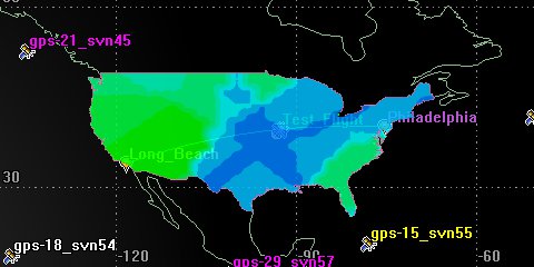
2D View: Dynamic contours for positional NavAcc
Single Object Coverage
Now, you need to perform a single object coverage analysis on the test flight to determine the PACC value along the actual path from Long Beach to Philadelphia. To evaluate the quality of coverage to a single object in STK, you can use the STK's Coverage capability. This capability is available for all types of vehicles, facilities, targets and sensors. Use the single-object coverage method to determine coverage if you are interested in coverage of a small number of well-defined locations or along the trajectory of a moving object.
The main differences between normal and single-object coverage are:
- Single-object coverage can be used to analyze objects with time-dependent positions.
- You can only analyze one figure of merit at a time using single-object coverage.
To determine the accuracy of the GPS position throughout Test_Flight’s flight, you need to assign the GPS satellites as assets for that object. To assess the quality of that coverage, in this instance, you would choose a navigation accuracy figure of merit type, then review the value of the PACC as Test_Flight flies from Long Beach to Philadelphia.
Assign Assets To a Single Object
To determine coverage for a single object, you must assign one or several assets to be used in coverage computations. For single-object coverage, it is important to have a clear understanding of the asset time periods. The time period for the coverage analysis is constructed as the interval of the reference object time period and the asset time period. Assets are used to calculate whether coverage to the object can be achieved. If you define a figure of merit for the coverage, coverage to the object from the assets is measured by the figure of merit values.
- Right-click on Test_Flight () in the Object Browser.
- Select the Coverage... (
 ).
). - Select GPSConstellation from the Assets list.
- Click .
- Click .
Define a Single Object Figure Of Merit
Position Accuracy (PACC) is a Navigation method that measures only the accuracy associated with the positional portion of the navigation solution. In your case, the portion you are interested in is the flight path for Test_Flight.
- In the Figure of Merit section, click .
- Set the following:
- Click to return to the Coverage Tool ().
- In the Figure of Merit section, take note of the Value: field value. This is the maximum value along Test_Flight's route.
| Option | Value |
|---|---|
| Type | Navigation Accuracy |
| Compute | Maximum |
| Method | PACC |
| Type | Over Determined |
| Time Step | 60 sec |
Report PACC
The FOM Value report shows the PACC value in meters at one minute intervals for the entire coverage interval. Create that now.
- In the Reports section, click .
- Does the data reflect what you saw when you computed PACC over the continental US airspace?
- Is it better? worse?
- Close the FOM Value report window.
Graph PACC
You can also graph the FOM value over time.
- In the Graphs section, click .
The graph shows how Test_Flight’s dilution of precision changes as it travels.
- Note the minimum and maximum FOM values.
- Leave the FOM Value graph open.
Single Object Contour Graphics
Now, let’s visualize the quality of coverage as Test_Flight flies from Long Beach to Philadelphia.
- Return to the Coverage Tool ().
- In the Graphics section, click .
- Set the following options:
- In the Level Attributes section, click .
- Enter the following values in the Level Adding area:
- Click .
- Enter the following values in the Level Attributes section:
- Click to return to the Coverage Tool ().
| Option | Value |
|---|---|
| Show Marker Animation Highlight | On |
| Show FOM Graphics on Vehicle Track | On |
Both of these options will allow the visualization to display in the Graphics windows.
| Option | Value |
|---|---|
| Add Method | Start, Stop, Step |
| Start | Integer below minimum FOM graph value |
| Stop | Integer above maximum FOM graph value |
| Step | 0.2 |
| Option | Value |
|---|---|
| Use Color Ramp | On |
| Select ramp colors | Blue in the first field, Red in the second field |
| Line Width | Thickest |
Get a Better Look
- Bring the 2D Graphics window to the front.
- Reset () the animation.
- Play () the animation.
Test_Flight’s route is colored to reflect the navigational accuracy at points along the flight.
As Test_Flight travels along it’s path his label color will also reflect the navigational accuracy at that point in time.
2D View: Contour graphics for Test Flight’s PACC
Your colors may be different from this view.
Change Your Perspective
- Bring the 3D Graphics window to the front.
- Zoom To Test_Flight ().
- Play () the animation.
Test_Flight’s object label and flight path also change color based on the PACC values in 3D.
3D View: Contour graphics for Test Flight’s PACC
De-Assign Assets
You just received a Notice of Advisory to Navstar Users (NANU) which states that GPS_23_SVN76 has been taken offline for some maintenance work. How will that impact your PACC values? Will you have to recreate your STK scenario? Fortunately, coverage objects allow you to keep an asset assigned but switch its status to inactive. This will essentially remove it from calculations. With GPS_23_SVN76 no longer in the picture, will you still meet your design criteria of never exceeding a PACC value of ten (10) meters?
Recompute PACC for Test Flight
Since you’re already looking at the aircraft’s route, let’s start with recomputing that.
- Return to the Coverage Tool ().
- Click the expand button (
 ) beside GPSConstellation to unnest the satellites.
 - Select gps_23_svn76 from the list.
- Select Inactive from the status drop-down menu below the Assets list.
- Click the button.
- In the Graphs section, click .
- Do you still meet your PACC requirements for this flight?
Inactive Multiple Satellites
Your maximum PACC has not decreased though some of your values might have changed slightly. This is because GPS is such a robust constellation. In order to receive a noticeable increase in PACC values, we will exclude several GPS satellites from our analysis.
- Bring the Coverage Tool () to the front.
- Click the expand button () beside GPSConstellation.
- Select all individually GPS satellites one through ten (1-10) from the list.
- Select Inactive from the status drop-down menu below the Assets list for each.
- Click the button.
- Bring the FOM Value graph to the front.
- Refresh your graph.
- Did your maximum PACC values increase noticeably?
- Do you still meet your PACC requirements for this flight?
- Close the FOM Value graph.
- Click to close to the Coverage Tool ().
If your FOM values have changed significantly, you may need to adjust your FOM contour values. Refer back to Single Object Contour Graphics for instructions on how to do this.
Recompute PACC for the Continental US
You have re-examined your PACC requirements for this flight, but what about the rest of the continental United States?
- Open ContUS_Cov’s () properties ().
- Select the Basic - Assets page.
- Click the expand button () beside GPSConstellation.
- Select GPS satellites one through ten (1-10) from the list.
- Select Inactive from the status drop-down menu beside the Assets list.
- Click .
Report Grid Stats Over Time
Let’s run a new Grid Stats Over Time report and see if the minimum and maximum static values for the figure of merit over the entire grid are still within your target range (PACC < 10).
- Open the Report & Graph Manager ().
- Select the following:
- Click .
- Did your maximum PACC values increase noticeably?
- Does the maximum static value for the figure of merit exceed ten (10) over some portion of the continental United States?
- Right-click the first time that the PACC maximum exceeds ten (10) in the My Grid Stats Over Time report.
- Open the Time context menu.
- Select Set Animation Time.
- Bring the 2D Graphics window to the front.
- Select the check box beside PACC in the Object Browser.
| Option | Value |
|---|---|
| Object Type | Figure of Merit |
| Object (Below Object Type) | PACC |
| Show Reports | On |
| Show Graphs | Off |
| Style | My Grid Stats Over Time |
| Generate as | Report/Graph |
Adjust the Display of Contours
Let’s update the FOM contours so that you can see where or if the PACC values exceed ten (10) because you won’t want to fly your aircraft in that area.
- Open PACC’s () properties ().
- Select the 2D Graphics - Animation page.
- Return to the My Grid Stats Over Time report.
- Scroll to the bottom of the report and note the minimum value.
- Return to the PACC's () properties ().
- In the Level Attributes section, click .
- In the Level Adding section, define the following:
- Click .
- Click .
| Option | Value |
|---|---|
| Start | value to an integer below minimum grid stats report value |
| Stop | 10 m |
| Step | .5 m |
Display the Legend Window
Next, let's display the legend window.
- Click .
- Click .
- In the 2D Graphics Window section, select the Show at Pixel Location check box.
- Click to dismiss the Figure of Merit Legend Layout window.
- Click .
Get a Better Look
- Bring the 2D Graphics window to the front.
- Reset () the animation.
The red on your map is where your position accuracy is over ten (10) meters based on setting the animation graphics from your report.
Change Your Perspective
- Bring the 3D Graphics window to the front.
- Zoom To United_States_of_America ().
- Use the mouse to zoom out until you can see the entire continental United States.
- Play () the animation.
- When you are finished, Reset () the scenario.
When You Finish
- Close the My Grid Stats Over Time report.
- Close the Report & Graph Manager ().
- Save () your work.