STK Premium (Space) or STK Enterprise
You can obtain the necessary licenses for this training by contacting AGI Support at support@agi.com or 1-800-924-7244.
The results of the tutorial may vary depending on the user settings and data enabled (online operations, terrain server, dynamic Earth data, etc.). It is acceptable to have different results.
An external file is needed for this training. You can download the zipped file from the SDF. If you are using STK Cloud, you can browse to the file: Sites -> AGI -> STK 12 -> Starter Tutorials -> DME_Session1_Constellation Concept Design and Trade Studies
Capabilities covered
This lesson covers the following STK Capabilities:
- STK Pro
- STK Analyzer
- STK SatPro
- STK Analyzer Optimization
- Coverage
Overview
Problem statement
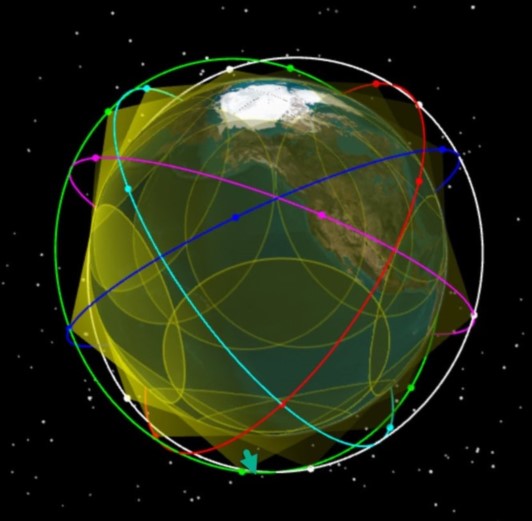
Across the industry, the digital engineering process is becoming more complex. Systems of systems are changing and updating in different stages of the mission life cycle. In this series, you will address these challenges by creating a fully connected digital thread with a common mission environment at the core. You will design and test a new satellite constellation for persistent, stereo coverage of hypersonic vehicles across the world. You will address this topic in stages: satellite constellations, hypersonic flight, EOIR synthetic sensors, communications links, and triggering events and systems. The vision is to integrate the mission environment and operational objectives into the digital thread early and throughout the entire product life cycle. Through digital mission engineering, you are now capable of quickly evaluating the overall mission impact of the smallest change to any component. This session will focus on the concept development phases using STK's Analyzer capability to conduct trade studies on the constellation geometry and optimizing based on system requirements.
Solutions
In this section of the DME series, you will focus on satellite constellation design using STK's Analyzer and Coverage capabilities. The goal in this exercise is to understand how to maximize the level of coverage with a global network of satellites. The main components you will analyze are the Revisit Time, which can be considered gap time, and the number of assets that have visibility to the ground. Using Analyzer's trade study capabilities, you can vary parameters of our system to find the most ideal configuration.
Upon completion of this tutorial, you will be able to:
- Build a Coverage analysis
- Design relevant Figure of Merit quality metrics
- Become familiar with the Analyzer work flow
- Understand constellation design configurations
- Load in external results file
Video guidance
Watch the following video. Then follow the steps below, which incorporate the systems and missions you work on (sample inputs provided).
Create a new scenario
In this scenario, you analyze the Number of Assets (NAsset) and how long the gaps are (RevisitTime). The goal is to maintain at least two assets while minimizing the gap time. You can start by building a scenario from scratch.
- Click the Create a Scenario (
 ) button.
 - Enter the following in the STK: New Scenario Wizard:
- When you finish, click .
- When the scenario loads, click Save (
 ). A folder with the same name as your scenario is created for you.
| Option | Value |
|---|---|
| Name | ImagingConstellation |
| Start | Default |
| Stop | Default |
Create a seed satellite to start the imaging constellation
The original satellite that is used to create the constellation is referred to as the “Seed” satellite. Use the Orbit Wizard to create the “seed” satellite from which the other satellites are derived.
- Insert a Satellite (
 ) using the Orbit Wizard (
 ) method.
 - When the Orbit Wizard opens, set the following:
- Click .
| Option | Value |
|---|---|
| Type | Circular |
| Satellite Name | seed_Satellite |
| Inclination | 50 deg |
| Altitude | 500 km |
| RAAN | 0 deg |
Adding a sensor to model visibility
The sensors in this study are for visualization purposes. You'd like to see what the satellites visability is over the Earth. You can model the sensor's large field-of-view to show where the sensor crosses the Earth.
- Using the Insert STK Objects tool, insert a Sensor (
 ) object using the Insert Default method.
 - When the Select Object window appears, select the satellite in the list and click .
Defining the sensor
Now that you have the sensor object in the scenario, define its properties.
- Open the sensor's () properties (
 ).
). - Go to the Basic - Definition page.
- Set the Cone Half Angle to 70 deg.
- Go to the 3D Graphics - Attributes page.
- Select the Translucent Lines check box.
- Set the Projection Translucency to 75.00.
- Select the 3D Graphics - Projection page.
- Set the Type to Earth Intersections.
- Click on the properties.
If you change the altitude of the satellite, you can visualize the line-of-sight intersection of the satellite to the Earth.
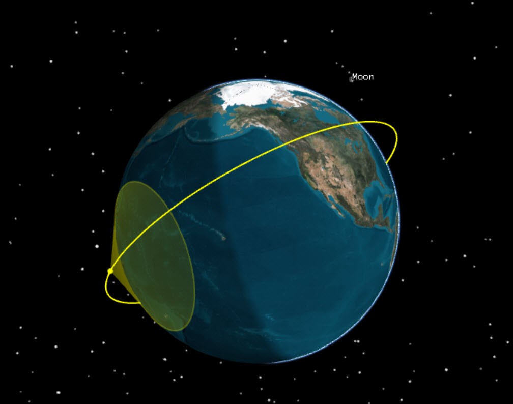
3D View: Satellite with sensor
Creating a Constellation
A Constellation object enables you to group satellites together. To get started, you can just include the seed satellite in the Constellation object.
- Insert a Constellation (
 ) using the Define Properties () method.
 - Ensure you are on the Basic - Definition page.
- Move (
 ) seed_Satellite to the Assigned Object field.
 - Click .
- Rename the constellation "Constellation".
Creating a Coverage analysis over the Earth
You are now ready to model a coverage analysis over the Earth. You can start by inserting a Coverage object and then you can define its properties.
- Insert a Coverage Definition (
 ) using the Define Properties () method.
 - Ensure you are on the Basic - Grid page.
- Set the following options:
- Leave all other defaults.
- Rename the CoverageDefinition to CoverageDefinition.
| Option | Value |
|---|---|
| Type | Latitude Bounds |
| Min Latitude | -60 deg |
| Max Latitude | 60 deg |
| Point Granularity | Lat/Long |
| Lat/Lon Value | 10 deg |
Assigning the Constellation
You set up the Coverage Definition object and now need to assign the seed satellite constellation to the coverage definition.
- Go to the Basic - Assets page.
- Select Constellation.
- Click .
- Select the Basic - Advanced page.
- Clear the Automatically Recompute Accesses option.
- Click .
Computing Coverage
- Right-click the Coverage Definition () in the Object Browser.
- Expand the CoverageDefinition menu.
- Select the Compute Accesses option.
Generating a Percent Coverage graph
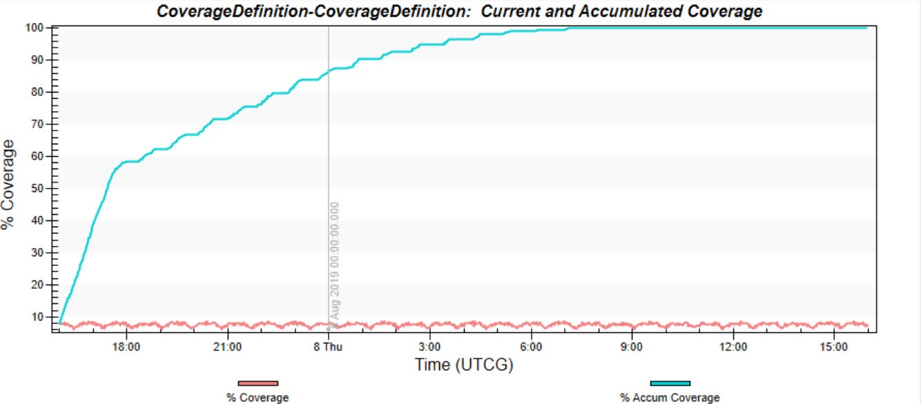
Now that you have set up and computed the coverage analysis, you can examine the quality of the coverage. But before you do that, take a quick look at the quality of the system you set up. One way to do that is to generate a Percent Coverage graph. This graph tells you how well the seed satellite is able to cover the globe throughout the scenario time period.
- Extend the Analysis menu.
- Select the
 Report & Graph Manager tool.
 - Set the Object Type to CoverageDefinition.
- Generate the Percent Coverage graph.
- Close the graph.
- Close the Report & Graph Manager.
Graph: Percent Coverage
Take a look at how the current coverage stays low throughout the analysis period, but how the accumulated coverage increases over time. This gives us an idea of how well the single seed satellite can cover the region. You can understand this further with the Figure of Merit object.
Designing the Figure of Merit
You just set up the problem with the Coverage object. To evaluate the coverage, you can use a Figure of Merit (FOM). Figure of Merit entities are a measure of the quality of coverage. In this study, you will focus on two parameters: Number of Assets and Revisit Time. The requirements state you must have at least two (2) assets covering every grid point at all times. You can use the N Asset FOM, which determines how many different assets are simultaneously covering each individual grid point at each time in the analysis period.
You can specify that the FOM compute the minimum value from the set of all grid points to make sure all grid points are at or above that threshold. Break down how to set this up.
- Insert a Figure of Merit (
 ) using the Define Properties () method.
 - When the Select Object window appears, select the CoverageDefinition in the list and click .
Defining the Figure of Merit for N Asset Coverage
You want to measure if at least two (2) satellites simultaneously cover every single point in the coverage analysis.
- Select the Basic - Definition page.
- Set the following options:
- Click .
- Rename the Figure of Merit to "NAsset".
| Option | Value |
|---|---|
| Type | N Asset Coverage |
| Compute mode | Minimum |
| Satisfaction | On |
| Satisfied If | At Least |
| Threshold | 2 |
Measuring the gap time
Now that the coverage has a threshold of at least two satellites per grid point, you can set up the gap time, or revisit time.
- Insert a Figure of Merit () using the Define Properties () method.
- When the Select Object window appears, select the CoverageDefinition in the list and click .
Defining the Figure of Merit for Gap Time
This Figure of Merit object measures the gap time. You want to minimize the gap time so that the maximum value satisfies the requirements in zero (0) second gap time.
- Select the Basic - Definition page.
- Set the following options:
- Click .
- Rename the Figure of Merit to "RevisitTime".
- Close the Insert Object tool.
| Option | Value |
|---|---|
| Type | Revisit Time |
| Compute mode | Maximum |
| Min # Assets | 1 |
| End Gaps | Include |
| Satisfaction | On |
| Satisfied If | At Most |
| Threshold | 0 sec |
Download precomputed trade study files
You are now ready to dive into some trade study analysis using Analyzer. You can build a simple example and then load the results into a more complex study. The goal is to become familiar with the Analyzer workflow as well as loading results of previously run analysis.
First, download the precomputed trade study files from the SDF. The steps are different if you are on your local machine or using STK Cloud. Choose the appropriate option below to download the files.
Option 1: Downloading the Files Locally
- Click the following link https://sdf.agi.com/share/page/site/AGI/folder-details?nodeRef=workspace://SpacesStore/32ef1e63-66e9-4486-afb1-2a211cfa0920
- Click Download as Zip on the right-hand side.
- Navigate to the zipped folder DME_Session1_Constellation Concept Design and Trade Studies.zip in your computer's Downloads directory.
- Unzip the folder if desired.
Option 2: Download the Files on STK Cloud
- Open a web browser in your STK Cloud session.
- Go to sdf.agi.com.
- Sign in to your account.
- Go to Sites -> AGI -> STK 12 -> Starter Tutorials.
- Place your cursor on the line that contains DME_Session1_Constellation Concept Design and Trade Studies.
- Select Download as Zip on the right side.
- Click the Gear icon in your STK Cloud browser window.
- Select Frame Explorer.
- Navigate to the zipped folder DME_Session1_Constellation Concept Design and Trade Studies.zip in Downloads directory.
- Unzip the folder if desired.
Setting up the analysis
You are now ready to dive into some trade study analysis using Analyzer. You can build a simple example and then load the results into a more complex study.
- Extend the Analysis menu.
- Extend the Analyzer menu.
- Select Analyzer (
 ).
).
Defining the input variables
Add the input variables to Analyzer.
- Select the seed_Satellite () in the STK Variables list.
- Select the Walker variable in the STK Property Variables General tab.
- Double-click the name to add it to the Analyzer Variables list. This brings over all the variables from this category.
- Expand the Propagator (J4Perturbation) variable.
- Double-click the SemiMajor Axis variable to add it to the Analyzer Variables.
Defining the output variables
Now that the input variables are defined, you can add the output variables. The output variables are the variables you'd like to solve for (Minimum N.Asset Overall and Maximum Revisit Time Overall).
- Expand the CoverageDefinition directory in the STK Variables list.
- Select the NAsset ().
- Expand the Overall Value directory.
- Double-click Minimum to add it to the Analyzer Variables list as an output.
- Select the RevisitTime ().
- Expand the Overall Value directory.
- Double-click Maximum to add it to the Analyzer Variables list as an output.
Computing a parametric study
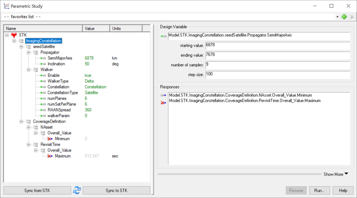
The trade study in this example varies the semimajor axis for a network of satellites. You can feed in the setup for the Walker analysis.
- Click the Parametric Study (
 ) button. This opens the Parametric Study dialog.
 - Click and drag the Semimajor Axis in the Components list to the Design Variables.
- Set the following options:
- Click and drag the desired response variables to the Responses section. The desired responses are:
- NAsset Minimum
- Revisit Maximum
| Option | Value |
|---|---|
| Starting Value | 6878 |
| Ending Value | 7678 |
| Number of samples | 9 |
| Step size | 100 |
Drag and drop the entire CoverageDefinition over to the desired response variables to quickly bring over all the parameters.
Defining the Walker variables
Define the walker parameters within the parametric study.
- Return to the Parametric Study window.
- Set the following for the Walker Constellation:
| Option | Value |
|---|---|
| Enable | True |
| Walker Type | Delta |
| Constellation | Constellation (you MUST type this exactly as it appears in the scenario) |
| ConstellationType | Satellite |
| numPlanes | 6 |
| numSatsPerPlanes | 6 |
| RAANSpread | 360 |
| walkerParem | 0 |
Your panel should looks similar to this:
Analyzer Panel with variables
Running the study
This study may take a few minutes to run. You can either run the study or load in the results from a precomputed study.
Option 1: Run the study
- Click .
- Now that the analysis is complete, examine the results.
You can watch as the 2D and 3D Graphics windows and the Timeline View change with each iteration.
Depending on the speed of your machine, this may take around ten (10) minutes without parallel computing. It can take longer depending on the machine.
Option 2: Load in a parametric study
- Extend the Analysis menu in STK.
- Extend the Analyzer menu.
- Select the Open Trade Study Result option.
- Browse to the DME_Session1_Constellation Concept Design and Trade Studies folder you downloaded from the SDF.
- Select DME_ParametricStudy.tstudy.
- Click .
- Examine the results.
In each of the runs, you should see the revisit time (gaps) decrease as the semimajor axis increases. Eventually it goes to zero. The average increases to two for the number of assets. The minimum number of assets eventually reaches two.
Generating a scatter plot
There are a few ways to view the data. One interactive way to view the data is in a 3D scatter plot.
- Use the Add View drop-down to select 3D Scatter Plot.
- Click .
- Set the following options:
- Click the graph to close the Dimensions window.
- Examine the matrix.
- Click any point to get information about that run.
| Option | Value |
|---|---|
| Dimensions | SemiMajorAxis(km) |
| X | Maximum |
| Y | Minimum |
| Z | SemiMajorAxis |
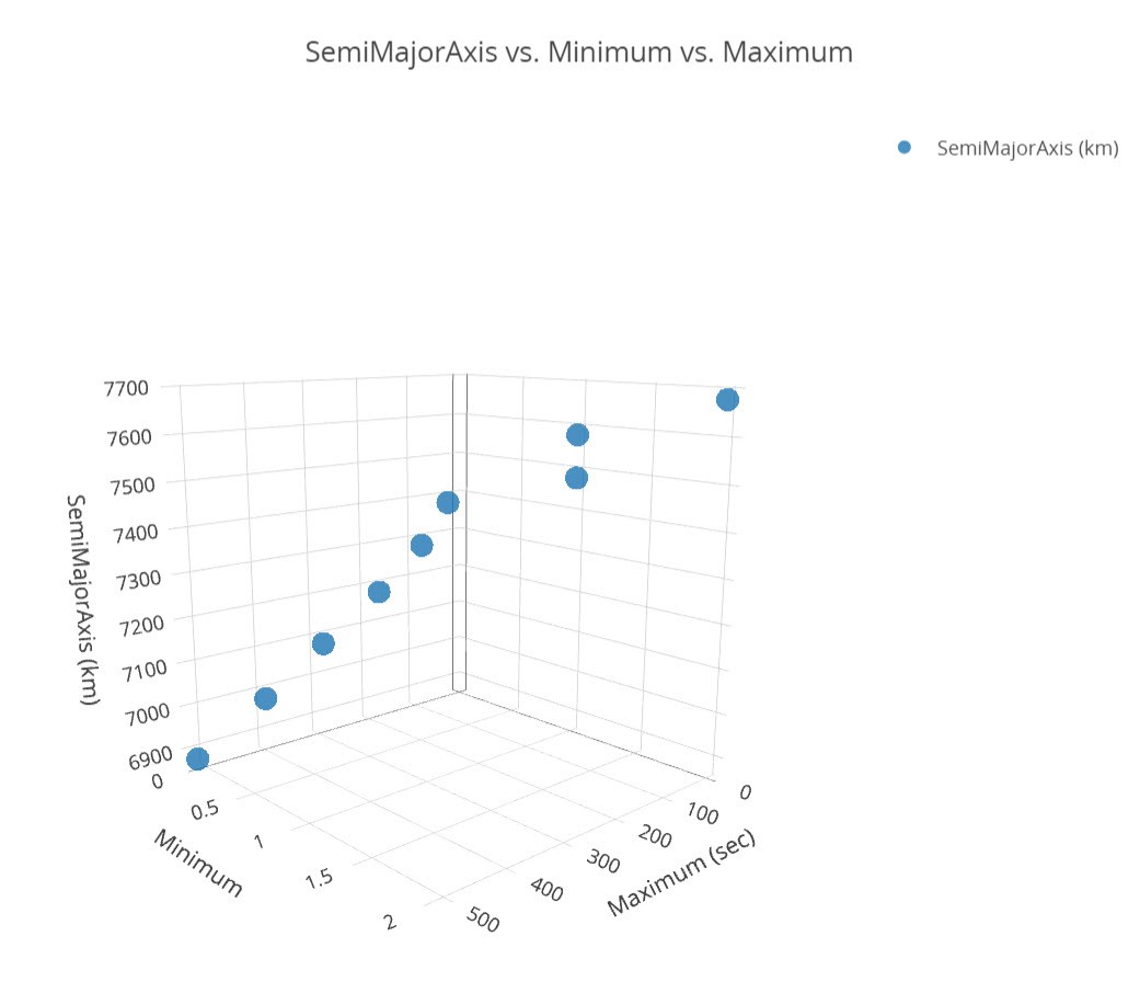
Analyzer 3D Scatter plot
Syncing to STK
Now all these criteria appear to meet in the final run (semi-major axis 7678 km), however, remember that the semimajor axis values are raised in 100 km increments. There is likely a minimum semimajor axis that enables you to achieve your goals sooner. If you consider cost, which might be tied to a higher orbit, you can find a lower semimajor axis that also reduces cost.
Push the results of a single run to STK and examine the scenario.
- Return to the Parametric Study window.
- Set the SemiMajorAxis to 7678 in the Components list. You do not need to enter units.
- Click . This pushes the results to STK. STK may take a few minutes to insert and configure the satellites.
- Close the Parametric Study window when the satellites are inserted.
Moving the satellites to the Constellation
Now that the Walker constellation is built, group the satellites into a Constellation object.
- Open the Properties () of Constellation ().
- Select Satellite in the Selection Filter. This selects all the satellites from the list.
- Move () the satellites to the Assigned Objects.
- Remove (
 ) seed_Satellite from the list. This object is already modeled as seed_Satellite11.
 - Click .
Recomputing the Coverage Definition
You should ensure the data is up to date. You can do that by recomputing the Coverage Definition.
- Right-click the CoverageDefinition () in the Object Browser.
- Extend the CoverageDefinition menu.
- Select Compute Accesses.
Examining the Data
Now that you have a result loaded in, look at some of the reports and graphs in STK that can shed some light on the scenario.
- Right-click NAsset () in the Object Browser.
- Select the Report & Graph Manager.
- Select the Percent Satisfied report in the Installed Styles list.
- Click .
- Generate the Grid Stats Over Time report.
You should have 100% coverage, which means you have a minimum of two (2) satellites with access to a point on the ground. The Percent Satisfied report confirms that information.
You can see that you meet the minimum, but you have quite a few locations that have five to six satellites with access. This creates a lot of redundancies, so you can start thinking of optimizing the setup.
You have two options at this point:
- Continue to test configurations using parametric scans, carpet studies, and design of experiments
- Optimize the scenario to find the optimal semimajor axis.
You may also consider if you need to change other factors with the study (number of satellites or planes). An optimization may take some time (4-10 hrs), so to speed things along, the results of the optimization test are available.
Loading in an optimization trade study
The study you are going to load in was run for many hours. The goal was to minimize the semimajor axis and the total number of satellites. At the same time, you want to minimize the revisit time (no gaps) and have two satellites maintain access with a point on the ground. Load in the data and examine it.
- Extend the Analysis menu.
- Extend the Analyzer menu.
- Select the Open Trade Study Result option.
- Browse to the DME_Session1_Constellation Concept Design and Trade Studies folder you downloaded from the SDF.
- Select DME_OptStudy.tstudy
- Click .
This opens the trade study results table and graph.
Proceeding if the 3D Scatter Plot fails to load
If the 3D scatter matrix fails to open, you can follow the steps below to create it.
- Use the Add View drop-down to select 3D Scatter Plot.
- Click the Dimensions button.
- Set the following options:
- Click the graph to close the Dimensions window.
- Examine the results of the graph. You can see the configurations that met the criteria in blue and those that didn't in gray.
- Click any point in the graph to see more information about a run.
- Examine the table.
| Option | Value |
|---|---|
| Dimensions | SemiMajorAxis(km) |
| X | Constraint (Maximum) |
| Y | Constraint (Minimum) |
| Z | SemiMajorAxis |
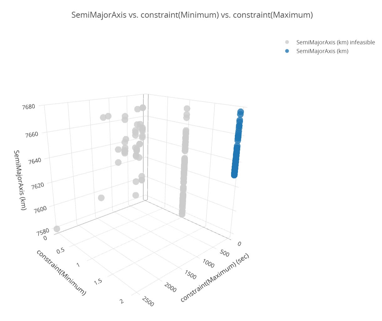
Analyzer 3D Scatter plot
You can scroll to see all the runs that were conducted and each result. You also have the option to export the data into Excel or another tool for post-processing. You can see the minimum semimajor axis value that meets all of the criteria is a value of 7629.9 km.
Setting up an optimization and sync to STK
This is an additional section for users who would like to setup an optimization themselves.
Looking at the data, there is a clear point that meets all the conditions for the study. Build the Optimizer to get an idea of the workflow. You will load in the best result from the data.
- Return to the Analyzer window.
- Click .
- Click . This loads the current setup in the scenario.
- Return to the Components list.
- Set the following:
| Option | Value |
|---|---|
| Enable | True |
| Walker Type | Delta |
| Constellation | Constellation (you MUST type this exactly as it appears in the scenario) |
| ConstellationType | Satellite |
| numPlanes | 6 |
| numSatsPerPlanes | 6 |
| RAANSpread | 360 |
| walkerParem | 0 |
Defining the semimajor axis
- Click and drag SemimajorAxis in the Components list to drop it in the Objective Definition - Objective field.
- Set the Goal to minimize.
Defining the NAsset Minimum
- Click and drag the NAsset Minimum in the Components list to drop it in the Constraints field.
- Set the Lower Bound to two (2).
- Click and drag the Revisit Time Maximum in the Components list to drop it in the Constraints field.
- Set the Lower and Upper Bounds to zero (0).
Defining the design variables
- Click and drag SemiMajorAxis in the Components list to drop it in the Design Variables field.
- Set the following Upper/Lower bounds:
| Option | Value |
|---|---|
| Lower Bound | 7578 |
| Upper Bound | 7678 |
Defining the number of satellites per plane
- Click and drag numSatsPerPlane in the Components list to drop it in the Design Variables field.
- Set the following options:
- Click .
| Option | Value |
|---|---|
| Start Value | 3 |
| End Value | 6 |
Defining the number of planes
- Click and drag numPlanes in the Components list to drop it in the Design Variables field.
- Set the following options:
- Click .
- Set the Algorithm to Darwin Algorithm.
| Option | Value |
|---|---|
| Start Value | 3 |
| End Value | 6 |
Pushing the results to STK
At this stage, you could run the optimization study. However, this is a time-consuming analysis. Instead of running the analysis, you can set the semimajor axis value to 7629.9 and push the results to STK.
- Set the SemiMajorAxis to 7629.9 in the Components list. You do not need to enter units.
- Click . This pushes the results to STK. It may take a minute to insert and configure the satellites.
Moving the satellites to the Constellation
Now that the Walker constellation is built, group the satellites into a Constellation object.
- Open the Properties () of Constellation ().
- Select Satellite in the Selection Filter. This selects all the satellites from the list.
- Move () the satellites to the Assigned Objects.
- Remove seed_Satellite from the list. This object is already modeled as seed_Satellite11.
- Click .
Recomputing the Coverage Definition
You should ensure the data is up to date. You can do that by recomputing the Coverage Definition.
- Right-click the CoverageDefinition () in the Object Browser.
- Extend the CoverageDefinition menu.
- Select Compute Accesses.
Examining the Data
Now that you have a result loaded in, let's look at some of the reports and graphs in STK that can shed some light on the scenario.
- Right-click NAsset () in the Object Browser.
- Select the Report & Graph Manager.
- Select the Percent Satisfied report in the Installed Styles list.
- Click.
- Return to the Report & Graph Manager.
- Select the Specify Time Properties radio button.
- Select the Use Step/size time bound radio button.
- Set the Step Size to one (1) second.
- Select the Grid Stats Over Time graph.
- Click .
You know from the results of the trade study that this configuration enables you to have a minimum of two (2) satellites with access to a point on the ground. This report confirms that you have 100% Satisfaction.
From this data, you see that you have full coverage throughout our mission. The minimum criteria of two satellites with simultaneous access to a grid point is met. This is confirmed in the Percent Satisfied Report and the Grid Stats Over Time graph. You can also see that you have a maximum of 4-6 satellites with simultaneous access to a grid point. This redundancy is key in case you lose a satellite in the course of a mission. The objective to create a new satellite constellation that provides persistent, stereo coverage of hypersonic vehicles across the world has been met.
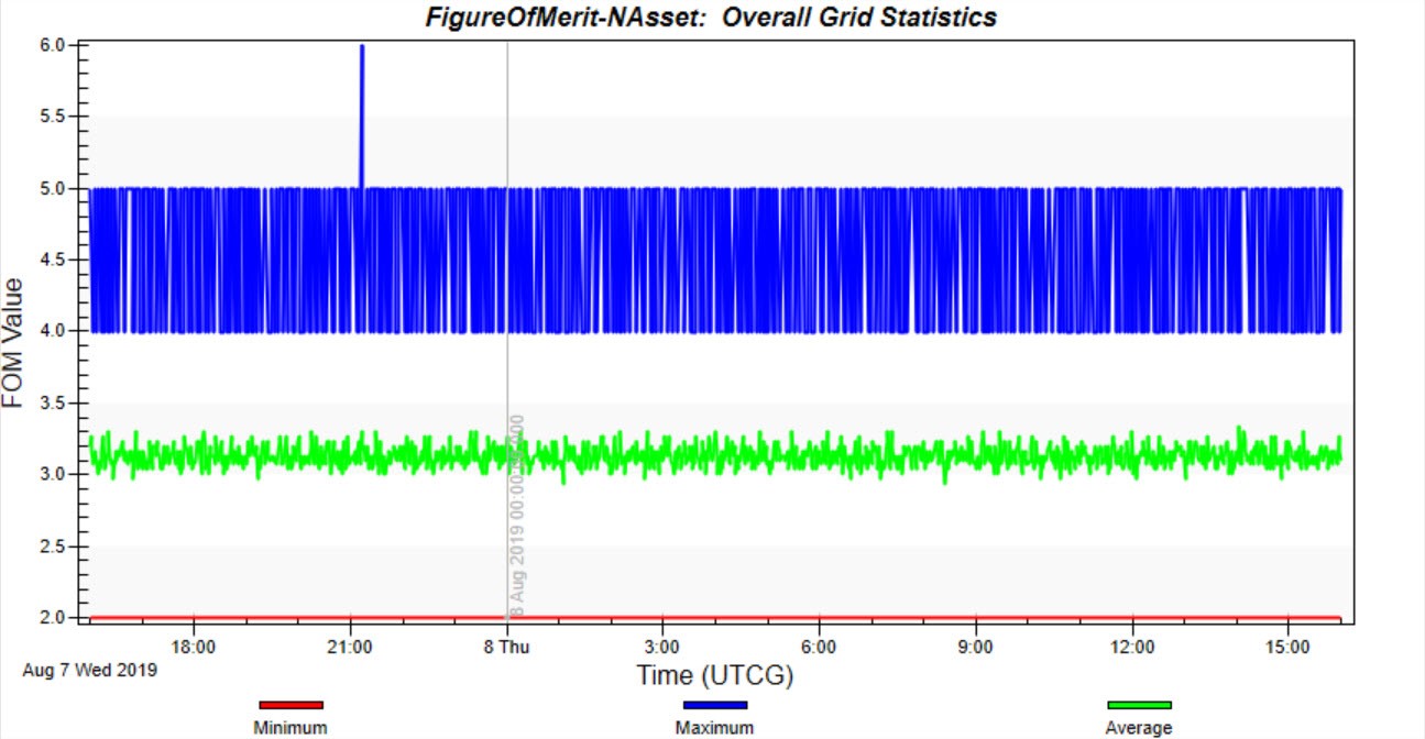
Graph: Percent Satisfied
Closing
You have the results of the optimization run, but there are many parameters that you can vary in the analysis. The flexibility of STK and Analyzer enables you to change an aspect of the mission (like the semimajor axis) while knowing that it carries through and is used in all calculations. If you have access to Model Center, you may link the analysis with Model Center and incorporate cost breakdowns, the total number of satellites, or any other parameters. You can integrate the mission earlier, thus considering all the factors in the environment.
DME Session 2
The next lesson in the DME series focuses on Hypersonics and EOIR. You will use a starter scenario and build your own hypersonic vehicle. You will use an EOIR sensor to image it. This leads up to the final session of the DME series where you bring the constellation from this lesson and the flight from session two together to understand how all components for the mission works together.