Strand Analysis
When a Chain is computed, all possible strands from the start object(s) to end object(s) through the specified connections are determined and times of valid access intervals are stored for each strand. The resultant intervals for each strand simply records when a start object can see an end object through the objects in that strand. The Chain Analysis options allows you to perform additional analysis for the computed strands in two ways:
- Optimal Strands: Using the computed strands, the Optimal Strands analysis computes the best strand(s) through the Chain based on a user specified metric for a set of specified times. For each time, a strand value is computed for each strand by computing a metric on each connection pair in a strand and then comparing or combining the pair-wise values to come up with an overall value for that strand. Strand values are then compared to determine which is best based on user specified criteria. You can specify metrics such as distance, data rate, duration, processing delay, or even use an AWB Calculation Scalar as the computed metric. In addition, you can specify the number of best strands to keep in memory. Keeping all data for all strands in memory could be both time and memory intensive so limiting the number stored to a small value will improve performance when computing and when animating.
- Network Throughput: While the Optimal Strand analysis can be used to determine the best paths through the computed strands of a Chain based on a metric, the Network Throughput can be used to compute the best overall instantaneous network data rate by summing all valid strand data rates. Strand data rates are based on the specified data rates for each object used in the Chain. The Network Throughput analysis uses a greedy algorithm based on strand ordering where all valid strands are ordered first by the minimum number of hops and then a user specified metric. Once ordered, strands contribute to the overall total throughput based on the minimum available data rate between connection pairs in each strand. Individual object data rate values are never exceeded. The resultant output of this analysis is the used strand data rates as well as each Chain objects used data rate.
For a Chain with many strands, it could be time consuming to evaluate strand analysis data at any requested time, especially during animation. For this reason, the analysis data is computed at sampled times determined by a specified time step.
The following options can be used to define the chain analysis data configuration:
| Option | Description |
|---|---|
| Compute | Compute optimal strands or network throughput. Chain accesses must be computed for the analysis data to be created. |
| # of Strands | (Optimal Strands only) Specify the maximum number of strands to store as “best.” Stored strands are ordered based on strand metric value and strand comparison type. |
| Metric | The computational metric to be evaluated for each valid strand at the sample times to determine the analysis results. |
| Strand Comparison | Comparison operator (min or max) used to compare the computed metric for two strands. |
Strand Analysis Metrics
STK has the ability to generate many, many metrics. For the strand analysis metric, you can use distance between objects in a strand, the duration of the access intervals within a strand, the data rate between objects in a strand, the processing delay of a strand or an access Analysis Workbench Calculation Scalar. Distance and processing delay metrics are summed across the connection pairs for a strand to compute an overall strand value. The data rate metric uses the minimum data rate between connection pairs for the overall strand value. Duration and Calculation Scalars are a bit more complicated.
The Duration metric can be used to select/compare strands for a given time by the longest (or shortest) duration over which the strands remain available. Once a strand is no longer valid based on time, all strands are evaluated for the current sample time to determine which strand now has the longest (or shortest) available duration. This metric can be used to minimize strand switching over a time period.
Calculation Scalar metrics can be used in two forms:
- an AWB file (*.awb) which is an exported access object Calculation Scalar
- a named built-in access object Calculation Scalar
When the strand metric computations are executed, each pair of objects in the strand is used to create a temporary access object behind the scenes and a Calculation Scalar of the specified type is created for that access. The Calculation Scalar is then evaluated to come up with a value of the metric for that pair of objects. The metric value is computed for each pair of objects defining the strand, then the values are combined using the Link Metric Comparison option (minimum, maximum, or sum) to come up with a value for the entire strand. Minimum values may be best for some metrics, such as distance, while maximum values may be best for others, such as signal strength. You can then specify the Strand Comparison option to use the minimum or maximum value of the strand metric to determine how strands are ordered in the analysis.
| Metric Options | Description |
|---|---|
| Data Rate | The minimum data rate between object pairs in a strand. The data rate from the "From Object" is used as the data rate for each Chain connection. The data rate can be specified for each object via the Chain Analysis options on the object or directly from the Basic Definition of a Transmitter object.
Data rate values are ignored for connections which have a common parent object, such as a Receiver/Transmitter pair on a common satellite object. |
| Distance | The summed distance between object pairs in a strand. Light time delay is not taken into account. |
| Duration | The time between the current sample time and the end time of a strand’s valid access interval. |
| Processing Delay | The summed time values of the processing delays specified by each object in the strand plus the light time delay between object pairs in the strand. The light time delay between object pairs is computed simply based on the objects’ positions divided by the speed of light. The first object’s processing delay is not included. |
| Scalar Calculation | An AWB Calculation Scalar along with a Link Metric Comparison operator (min, max, sum) can be used as the metric to evaluate the value of a strand. The Calc Scalar must be valid for an Access object as the metric is evaluated on each sequential pair of objects in the strand. The link metric comparison operator is then used to compare each object pair’s computed metric to come out with an overall value for the strand. The Calculation Scalar can be specified using a file from an exported Access object Calculation Scalar or as the name of a built-in Access Calculation Scalar. |
If the Calculation Scalar is not valid for any used connections in your Chain, the strand analysis data cannot be computed and an error message is displayed in the Message Viewer.
| Scalar Calculations Options | Description |
|---|---|
| File | Specify the Analysis Workbench file (.awb) file to be used as the metric when evaluating object pairs. |
| Name | Specify the Analysis Workbench built-in access Calculation Scalar to be used as the metric when evaluating object pairs. |
| Link Metric Calculation | Method used to evaluate object pair metric values when computing an overall strand metric from its constituent strand object pairs. The min, max, or sum of object pair metric values may be specified as the overall strand value. |
Create an Analysis Workbench File (*.awb)
To create an Analysis Workbench file (*.awb) that can be used as a metric for strand analysis calculations, you can create an access between two objects that represent similar objects to the objects in your Chain connections. Then in the Analysis Workbench tool, create a Calculation Scalar for the metric you want to compute with and export it. The access object can be deleted; it is not needed for the actual Chain computations. When the strand analysis is computed, a temporary Calculation Scalar is created by importing this file for each of the object pairs in the strand and deleted when the computation is done.
To discover the built-in Calculation Scalar names, it’s easiest to create a temporary access between two objects that represent similar objects to the objects in your Chain connections.
- In the AWB tool, select the Calculation tab.
- Select the access object you just created. You will see the available built in components.
- Look at the tooltip for a Calculation Scalar component and use the name next to the label “Scalar Calculation Name” as the metric name.
- Delete the temporary access object.
When the strand analysis is computed, a temporary Calculation Scalar is created with this built-in type for each of the object pairs in the strand and deleted when the computation is done.
Strand Analysis Time Samples
All strand analysis data is stored at sampled times based on the input sample time step. For very large Chains, it would not be possible to store all data for all strands or be able to compute the optimal strand or network throughput data on the fly while animating.
| Scalar Calculations Options | Description |
|---|---|
| Sampling Timestep | Time step referenced from the animation start time to compute the strand analysis data. |
| Include Strand Access Edge Times | Specify whether to include all start and stop access times from all valid strands in addition to the sampled timesteps. |
To aid in making sure the visualized analysis data is accurate for the current animation time, sample times for computations are referenced to the start animation time. Including strand access end times will add the start and stop access times from all valid strands into the sampled times. This option can lead to the sampled data having many additional sample times computed and stored, especially for Chains with many valid strands. While the option can cause a large amount of memory to be used and lead to a much slower calculation of strand analysis data, it does ensure that reported interval data will be exact.
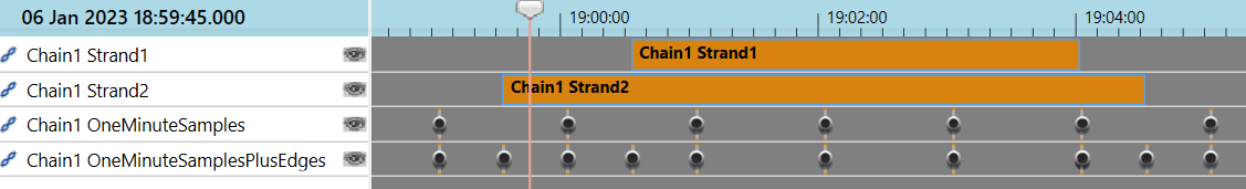
The timeline view below shows the effect of including and not including strand edge times when performing an optimal strand analysis. The behavior would be the same for network throughput data. Chain1 has two valid strands with optimal strands computed at one (1) minute intervals. If samples are taken without edge times, for the animation time in the timeline view image (where the vertical line is, 18:59:45), there will be no valid optimal strands displayed since the last computed sample time is used to choose which optimal strand to display. At the animation time of 18:59:45, the optimal strand sample time of 18:59:00 is used, which has no valid strands.
If the edge times are included, a valid strand (18:59:30) will be displayed. Problems can still occur even with edge times included as shown when the animation time is at the end of Strand2. If the animation time is between the last time of the interval time (19:04:30) and the next sample time (19:05:00), an optimal strand may attempt to be displayed, but there really isn’t a valid strand. STK detects this problem and doesn't display any best strands in this case, but there are times when the wrong best path may be displayed. For this reason, it is important to keep the animation time in sync with the sample times.
Example of an optimal strand analysis
As a hypothetical example, suppose you have a Chain with two valid strands where you want to evaluate the best path based on some metric:
- Place1 -> Satellite1 -> Place2
- Place1 -> Satellite2 -> Place2
Let’s use a calculation scalar to simulate the shortest path (even though we have a hard-coded metric of distance) so you use the built-in metric name: From-To-AER(Body).Cartesian.Magnitude.
If you hypothetically (completely notional) say the pair distances for a given time are evaluated as follows:
| Connection | Pair |
|---|---|
| Place 1 -> Satellite 1 | 10 km |
| Satellite 1 -> Place 2 | 70 km |
| Place 1 -> Satellite 2 | 20 km |
| Satellite 2 -> Place 2 | 40 km |
Given the object pair metric values for the connection pairs above, an overall metric value can be assigned to each strand depending on the link comparison operator. The table below shows the possible strand values for the different link operator option:
| Strand | Minimum Link Distance | Maximum Link Distance | Sum of Link |
|---|---|---|---|
| Place 1 -> Satellite 1 -> Place 2 | 10 km | 70 km | 80 km |
| Place 1 -> Satellite 2 -> Place 2 | 20 km | 40 km | 60 km |
After the strand values are computed based on the connection pair metric values and the link metric comparison setting, the individual strands are compared to find the “best strand.” The following tables shows what would be computed as the “best” strand based on the link comparison and the strand comparison options:
| Strand Comparison | (Link comparison operator = min) | (Link comparison operator = max) | (Link comparison operator = sum) |
|---|---|---|---|
| Min | Place 1 -> Satellite 1 -> Place 2 | Place 1 -> Satellite 2 -> Place 2 | Place 1 -> Satellite 2 -> Place 2 |
| Max | Place 1 -> Satellite 2 -> Place 2 | Place 1 -> Satellite 1 -> Place 2 | Place 1 -> Satellite 1 -> Place 2 |