STK Premium (Space) or STK Enterprise
You can obtain the necessary licenses for this tutorial by contacting AGI Support at support@agi.com or 1-800-924-7244.
Usage of the Sparse Nonlinear Optimizer (SNOPT) search profile requires an additional license. Please contact AGI support for licensing.
The results of the tutorial may vary depending on the user settings and data enabled (online operations, terrain server, dynamic Earth data, etc.). It is acceptable to have different results.
Capabilities covered
This lesson covers the following capabilities of the Ansys Systems Tool Kit® (STK®) digital mission engineering software:
- STK Pro
- Astrogator
- Analysis Workbench
Problem statement
Engineers and operators want to transfer a spacecraft from a low Earth orbit (LEO) to a geosynchronous orbit (GEO) along a spiral path using a low-thrust maneuver. "Low" may be a relative term, but in space travel, there is a boundary for what is considered "low thrust": an acceleration of 10-3m/s2 or lower. Most systems that use this type of propulsion are electric propulsion systems. Maneuvers at this acceleration are designed for long missions and can be effected on a scale of months. They may not be fast, but they are efficient. Given the planned length of the mission, you want to ensure that the maneuver effecting the orbital plane change is optimized for the most feasible efficiency.
Solution
Use the STK/Astrogator® capability, a SNOPT (Sparse Nonlinear OPTimizer) search profile, and the Analysis Workbench capability's Vector Geometry tool to transfer a satellite from LEO to GEO along a spiral path with an Optimal Finite Maneuver.
What you will learn
Upon completion of this tutorial, you will be able to:
- Model a low-thrust orbit
- Design a low-thrust Finite Maneuver
- Build the steps for an Optimal Finite Maneuver using a SNOPT search profile
- Calculate an Optimal Finite Maneuver using a Finite Maneuver as an initial guess
- Import and export Collocation Node files
- Calculate an Optimal Finite Maneuver using an Initial Guess file
Creating a new scenario
Before you begin with any analysis, you need to create a two-day scenario.
- Launch the STK application (
 ).
). - Click
 Create a Scenario.
 - Enter the following in the STK: New Scenario Wizard:
- Click when you finish.
- Click Save (
 ) when the scenario loads.
 - Verify the scenario name and location when the Save As dialog box opens.
- Click .
| Option | Value |
|---|---|
| Name | Spiral_to_GEO_Optimal_Finite |
| Analysis Start Time | Default |
| Analysis End Time | + 2 days |
A folder with the same name as your scenario is created for you.
Save (![]() ) often!
) often!
Configuring your workspace
Your exercise will focus primarily on the 3D Graphics window.
- Close the 2D Graphics window.
- Close the Timeline View.
Creating a new Astrogator satellite
Add a satellite to the scenario and select Astrogator as the propagator to utilize the Astrogator capability for trajectory and maneuver planning.
Adding a new Satellite object
Insert a new Satellite object into your scenario.
- Bring the Insert STK Objects tool (
 ) to the front.
 - Select Satellite (
 ) in the Select an Object To Be Inserted list.
 - Select the Insert Default () method.
- Click .
- Rename Satellite1 () Finite_Maneuver.
Changing the propagator to Astrogator
There are several types of
- Right-click on Finite_Maneuver () in the Object Browser.
- Select Properties (
 ) in the shortcut menu.
 - Select the Basic - Orbit page when the Properties Browser opens.
- Open the Propagator drop-down list.
- Select Astrogator.
- Click to confirm your change and to keep the Properties Browser open.
Creating a custom Engine Model component
Before you dive into building the Mission Control Sequence (MCS) using the Astrogator capability, you must first define the custom low-thrust engine model you will use with the satellite. You can do so using the
Duplicating a prebuilt component
Duplicate an existing read-only
- Click Component Browser (
 ) on the MCS toolbar.
 - Select the Engine Models (
 ) folder in the Show Component Type list when the Component Browser dialog box opens.
 - Select Constant Acceleration and Isp (
 ) in the Engine Models list.
 - Click Duplicate component (
 ) on the Engine Models toolbar.
 - Enter My Engine in the Name field when the Field Editor dialog box opens.
- Click to create the new Engine Model component and to close the Field Editor dialog box.
The Constant Acceleration and Isp Engine Model employs constant values for acceleration and Isp. At each time step, the model adjusts the thrust to hold acceleration and Isp constant given a changing mass.
Customizing the engine component
Now that you have created a duplicate component, you can customize its acceleration, specific impulse (Isp), etc.
- Select My Engine (
 ) in the Engine Models list.
 - Click View properties () on the Engine Models toolbar.
- Double-click on Acceleration in the Name column when the My Engine dialog box opens.
- Enter 9.8 cm/sec^2 in the Real Number field when the Real Number Field dialog box opens.
- Click to confirm your change and to close the Real Number Field dialog box.
- Double-click on Isp in the Name column.
- Enter 3000 s in the Real Number field when the Real Number Field dialog box opens.
- Click to confirm your change and to close the Real Number Field dialog box.
- Click to confirm your changes and to close the My Engine dialog box.
- Click to confirm your changes and to close the Component Browser.
The Earth surface gravity acceleration for Isp conversions (g) is 0.00980665 km/sec^2. This looks similar to the Acceleration value you are entering, which is equivalent to 0.000098 km/sec^2. Be sure you are editing the Acceleration value and not the g value for your engine model.
Configuring the satellite's initial state
The default segments in the MCS are Initial State and Propagate. Starting with the initial state, you can define the segments to build the low-thrust sequence.
- Return to the Properties Browser.
- Select Initial State (
 ) in the MCS.
 - Select the Elements tab.
- Open the Coordinate Type drop-down list.
- Select Keplerian.
- Set the following options:
- Keep the remaining default values.
- Click to confirm your changes and to keep the Properties Browser open.
| Option | Value |
|---|---|
| Semi-major Axis | 7000 km |
| True Anomaly | 140 deg |
Modeling a Finite Maneuver
Next, define a Finite Maneuver segment. A Finite Maneuver is effectively a Propagate segment with thrust. It uses a defined propagator to propagate the state, accounting for the acceleration due to thrust. The selected engine model specifies the magnitude of the thrust vector and the selected attitude control specifies the direction of the thrust vector. Like Propagate segments, each calculated point is added to the ephemeris, and propagation continues until Astrogator reaches a stopping condition.
Thanks to the initial state, you have a starting model for the orbit. You can use a Finite Maneuver to model the effects of applying thrust to the satellite and provide data to "seed" for an optimized maneuver later in the lesson.
Inserting a Maneuver segment
Insert a
- Select Initial State () in the MCS.
- Click Insert Segment After (
 ) on the MCS toolbar.
 - Select Maneuver (
 ) when the Segment Selection dialog box opens.
 - Click to confirm your selection and to close the Segment Selection dialog box.
Configuring the Maneuver segment
Configure the Maneuver segment for a Finite Maneuver, then configure how the maneuver pointing and the spacecraft's attitude are updated.
- Open the Maneuver Type drop-down list.
- Select Finite.
- Click the Finite Propagator and Force Model for Optimization ellipsis (
 ).
). - Select Earth Point Mass () when the Select Component dialog box opens.
- Click to confirm your selection and to close the Select Component dialog box.
Using the Earth Point Mass Propagator component will reduce the computational time, while still providing useful results.
Setting the attitude
The "thrust vector" describes the direction of acceleration applied to a satellite.
- Select the Attitude tab.
- Open the Attitude Control drop-down list.
- Select Thrust Vector.
- Ensure the Attitude Update is set to Update during burn.
With this attitude control setting, the Delta-V vector is specified in some reference frame, using either Cartesian or spherical components. Astrogator then computes the attitude so that the total thrust vector in the body frame, as specified by the thruster set or engine model, aligns with this vector in the reference axes.
With this option, the maneuver pointing is updated throughout the maneuver in order to maintain the required thrust direction in the specified direction at every instant throughout the burn. Therefore, the thrust vector rotates with the specified coordinate system.
Defining the thrust axes
When you create a maneuver, you need to define the direction in which to apply thrust. In this situation, you don't want to incorrectly choose axes that take you back to Earth. Your goal is to reach a higher orbit. The axes you will use are the In-Track, Cross-Track, Radial (ICR) axes with a Z axis along position vector and an X axis toward inertial velocity vector. This is also known as an ICR frame. Using this frame, you can align and constrain the position and velocity vectors along the trajectory of the satellite. These axes are available as a preinstalled template file, available as part of the Analysis Workbench capability's
- Click the Thrust Axes ellipsis ().
- Ensure that the Filter By option is set to Templates when the Select Reference dialog box opens.
- Select Satellite () in the objects list.
- Select ICR (
 ) in the Installed Templates () folder in the Templates for Satellite list.
 - Click to confirm your selection and to close the Select Reference dialog box.
Defining the spherical components
You have the option to define the direction of the thrust axis in either Cartesian or spherical components. Either way, you will be able to compute your final solution. Some people, however, find spherical components easier to understand.
- Ensure the Spherical option is selected.
- Enter 42 deg in the Azimuth field.
- Enter 27 deg in the Elevation field.
- Click to confirm your changes and to keep the Properties Browser open.
Selecting the Engine Model component
Using the Engine Model component you previously created, you can define the magnitude and nature of the propulsion.
- Select the Engine tab.
- Ensure the Engine Model option is selected in the Propulsion Type panel.
- Click the Engine Model ellipsis ().
- Select My Engine () when the Select Component dialog box opens.
- Click to confirm your selection and to close the Select Component dialog box.
Defining the stopping condition
Your satellite models the maneuver up until a specified stopping condition.
- Select the Propagator tab.
- Enter 18 hr in the Trip Value field.
- Click to confirm your change and to keep the Properties Browser open.
Defining the Propagate segment
After the maneuver, you want to model the rest of the orbit. You can do that by updating the Propagate segment following the Maneuver segment.
- Select Propagate (
 ) in the MCS.
 - Click the Propagator ellipsis ().
- Select Earth Point Mass () when the Select Component dialog box opens.
- Click to confirm your selection and to close the Select Component dialog box.
- Note the default Duration stopping condition.
- Enter 24 hr in the Trip field.
- Click Segment Properties () on the MCS toolbar.
- Open the Color drop-down list when the Edit Segment dialog box opens.
- Select a color that's different from the Maneuver segment.
- Click to confirm your selection and to close the Edit Segment dialog box.
- Click to confirm your changes and to keep the Properties Browser open.
The Finite Maneuver and Propagate segments can be viewed in the 3D Graphics window. By selecting different colors, you can see when each segment takes place after running the mission control sequence.
Running the Mission Control Sequence
To calculate the trajectory of the spacecraft, you must run the Mission Control Sequence.
- Click Run Entire Mission Control Sequence (
 ) on the MCS toolbar.
 - Close the Properties Browser.
- Bring the 3D Graphics window to the front.
- Save () your scenario.
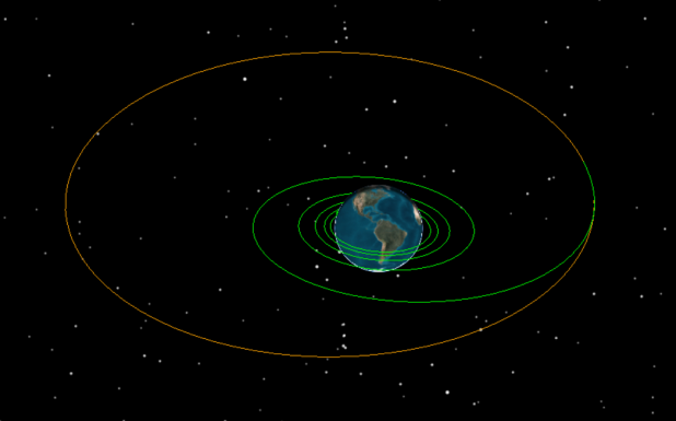
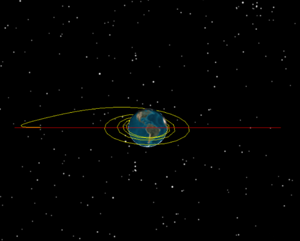
propagated Finite Maneuver
You can see that your maneuver got your satellite close to GEO.
Generating a Maneuver Summary report
Create a
- Right-click on Finite_Maneuver () in the Object Browser.
- Select Report & Graph Manager... (
 ) in the shortcut menu.
 - Expand (
 ) the Installed Styles () folder in the Styles panel list when the Report & Graph manager opens.
 - Select the Maneuver Summary (
 ) report.
 - Click .
- Take note the Duration of the burn as well as the total Delta V and Fuel Used.
- Keep the Maneuver Summary report and the Report & Graph Manager open.
While your maneuver did get you close to GEO, you can do better. For that, you can use a Optimal Finite Maneuver.
Using an Optimal Finite Maneuver with SNOPT
You want the spacecraft to travel from LEO to GEO. With an
A
There are two approaches you can take to optimize your maneuver: the first is to compute the Finite Maneuver and use the solver, which is time intensive; the other is to use an Initial Guess file. Since you already computed the Finite Maneuver, you can reuse those steps first.
For more information on initial guesses for Finite Maneuver optimization, refer to the Astrogator
Using a Finite Maneuver trajectory as an initial guess
While your initial solution was not ideal, it got you close to GEO. Now, you can begin solving for a solution. You can use the Finite Maneuver trajectory as the initial guess, or "seed," in the computation. The Finite Maneuver provides Astrogator with some data to start. The advantage to seeding from a Finite Maneuver without a node file is that you can "start from scratch" within Astrogator. This is useful when you don't have a means for producing a node file or you're less familiar with the problem, and builds on Astrogator's inherent interactive design environment paradigm.
Creating a new satellite
Copy the existing Finite Maneuver satellite and propagate the initial Finite Maneuver.
- Select Finite_Maneuver () in the Object Browser.
- Click Copy (
 ) on the Object Browser toolbar.
 - Click Paste (
 ) on the Object Browser toolbar to create a copy of Finite_Maneuver ().
 - Rename Finite_Maneuver1 () Optimal_Finite.
- Clear the check box for Finite_Maneuver () in the Object Browser to clear it from displaying in the 3D Graphics window.
Propagating the Finite Maneuver
Prior to setting up your Optimal Finite Maneuver, re-run the MCS to propagate your Finite Maneuver.
- Open Optimal_Finite's () Properties ().
- Select the Basic - Orbit page when the Properties Browser opens.
- Click Run Entire Mission Control Sequence () to recreate the same Finite Maneuver.
Before you can seed an Optimal Finite Maneuver from a Finite Maneuver, the Finite Maneuver's state must already be propagated by the selected Maneuver segment. This is why you must ensure you run your MCS first.
Changing the Maneuver segment's color
Update the color of the Maneuver segment.
- Select Maneuver () in the MCS.
- Click Segment Properties () on the MCS toolbar.
- Open the Color drop-down list when the Edit Segment dialog box opens.
- Select a color that's different from Finite_Maneuver's () Maneuver () and Propagate () segments.
- Click to confirm your selection and to close the Edit Segment dialog box.
Selecting an Optimal Finite Maneuver segment
Change the Maneuver type from Finite to Optimal Finite.
- Confirm Maneuver () is selected in the MCS.
- Open the Maneuver Type drop-down list.
- Select Optimal Finite.
- Note that the tabs have changed.
The tabs you saw before were Attitude, Engine, and Propagator; you should now see Solver and Engine.
Setting the number of nodes
To compute the Optimal Finite Maneuver, you must break up the trajectory of the satellite so that it can be computed in sections specified by nodes. Nodes are states along the trajectory arc that serve as control points for the direct transcription algorithm. The nodes are adjusted by the optimizer to best satisfy the thrust-augmented dynamics. For this calculation, you will use 120 nodes. This value was settled upon after running the analysis at:
- 30 nodes
- 60 nodes, which provided sufficient results
- 120 nodes, which provides sufficient results and a smooth trajectory
- Higher node values, which provided sufficient results, but without much improvement in the analysis
If you were working on your own mission, you would go through this same iterative process to find the appropriate value.
- Select the Solver tab.
- Enter 120 in the Number of Nodes field in the Problem Setup panel.
- Click .
- Open the Scaling Options drop-down list when the Algorithm Options dialog box opens.
- Select Scale based on initial state.
- Click to confirm your selection and to close the Algorithm options dialog box.
- Click to confirm your changes and to keep the Properties Browser open.
Scaling typically improves the numerical behavior of optimization problems. This option specifies how to accomplish scaling.
Defining the Seed options
The solution of an Optimal Finite Maneuver problem requires an
- Select the Seed from - Finite Maneuver option in the Problem Setup panel.
- Click .
- Note the Node Status has been updated to 120 nodes seeded from finite maneuver and that two additional tabs have been exposed: Log and Steering/Nodes.
This loads in the values from the Finite Maneuver.
The orbit states, mass, and the thrust attitude for an Optimal Finite Maneuver are ultimately solved for at a set of discrete time nodes, suitably placed between maneuver start and end times (which themselves may be variables). It is precisely at these nodes that the initial guess states and controls are also sampled after seeding is accomplished.
For more information on seeding an Optimal Finite Maneuver from a finite maneuver, refer to the Astrogator
Reviewing the Initial Boundary conditions
Next you want to limit what values your optimal finite calculation can use. This will keep your values between reasonable conditions. In the case of the Initial Boundary, you will just check the values.
- Click .
- Take a look at the variables when the Initial Boundary Conditions dialog box opens. You won't change any values, only review the numbers.
- a — corresponds to the semi-major axis
- h & k — describe the shape of the satellite's orbit and the position of perigee
- p & q — describe the orientation of the satellite's orbit plane
- L — corresponds to the Mean Longitude
- Click to close the Initial Boundary Conditions dialog box without making any changes.
For more information on these parameters, review the Equinoctial Coordinate Type help page.
Defining the Final Boundary conditions
You can use the Final Boundary to define the upper and lower bounds for the orbital parameters you want for the final state.
- Click .
- Clear the Set from Initial Guess check box when the Final Boundary Conditions dialog box opens.
- Set the following values in the Set Explicitly panel. Set the upper bound first, then the lower bound, one variable at a time:
- Click to confirm your changes and to close the Final Boundary Conditions dialog box.
- Click to confirm your changes and to keep the Properties Browser open.
| Lower Bound | Variable | Upper Bound |
|---|---|---|
| 42000 km | a | 42000 km |
| 0 | h | 0 |
| 0 | k | 0 |
| 0 | p | 0 |
| 0 | q | 0 |
| 0 deg | L | 1800 deg |
| Tf - 7200 sec | Final Time | Tf + 7200 sec |
If your lower bound value is higher than the upper bound, you will see an error (![]() ). That's why it's a good idea to set the upper bound first.
). That's why it's a good idea to set the upper bound first.
Defining the Path Boundaries
The Path Boundaries enable you to define the upper and lower bounds of the orbital states and the thrust spherical angles (when not using unit vectors as controls in the Algorithm Options) on the trajectory at all but the initial and terminal points.
- Click .
- Clear the Compute from Initial Guess check box when the Path Boundaries for Variables dialog box opens.
- Set the following values in the State Element Variables panel. Set the upper bound first, then the lower bound, one variable at a time:
- Click to confirm your changes and to close the Path Boundaries for Variables dialog box.
- Click to confirm your changes and to keep the Properties Browser open.
You can explicitly set some values. In the following steps, you can set the goal for the satellite to go from the LEO regime to a final GEO position with an inclination and eccentricity of zero (0).
| Lower Bound | Variable | Upper Bound |
|---|---|---|
| 6000 km | a | 65000 km |
| -0.9 | h | 0.9 |
| -0.9 | k | 0.9 |
| -0.9 | p | 0.9 |
| -0.9 | q | 0.9 |
| 140 deg | L | 1800 deg |
Specifying the maneuver optimization objective
Specify the maneuver optimization objective to minimize the amount of fuel used.
- Click in the Problem Execution panel.
- Open the Objective drop-down list when the SNOPT Options dialog box opens.
- Select Minimize propellant use.
- Click to confirm your selection and to close the SNOPT Options dialog box.
- Click to confirm your changes and to keep the Properties Browser open.
This determines the thrust attitude program (and any other optimizable variables) to minimize the net propellant mass expended over the maneuver duration. When you select this option, Astrogator effectively maximizes the propellant mass at the maneuver final time.
Setting the Run Mode to Optimize via direct transcription
Set the Run Mode to Optimize via direct transcription. Running the sequence with this option initiates the Finite Maneuver optimization process.
- Open the Run Mode drop-down list in the Problem Execution panel.
- Select Optimize via direct transcription.
- Note that the Halt MCS and Discard Result if Optimization is Unsuccessful check box has been automatically selected.
- Click to confirm your change and to keep the Properties Browser open.
When selected, if the numerical optimizer indicates unsuccessful convergence to a locally best solution, the MCS stops and the result from the direct-transcription-collocation system is not stored or available for further use.
For more information on maneuver optimization using direct transcription methods, refer to the Astrogator
Confirming the Engine model component
Before you run this model, confirm that you are using the correct Engine Model component.
- Select the Engine tab.
- Confirm the Engine Model is set to My Engine in the Propulsion Type panel.
- Confirm the Pressure mode is set to Pressure-Regulated.
- Confirm that the Thrust Efficiency is 1.
- Confirm that the Thrust is set to Affects Accel Only.
If you click the Log tab, you will see data only when the analysis has been run. If you click the Steering/Nodes tab, you will see a table of data on each of the 120 nodes. The Azimuth and Elevation columns have values taken from the Finite Maneuver.
Updating the Propagate segment's color
Change the Propagate segment's color.
- Select Propagate () in the MCS.
- Click Segment Properties () on the MCS toolbar.
- Open the Color drop-down list when the Edit Segment dialog box opens.
- Select a color that's different from Finite_Maneuver's () Maneuver () and Propagate () segments.
- Click to confirm your change and to keep the Properties Browser open.
- Save () your scenario.
Running the MCS for the Optimal Finite Maneuver
With your MCS configured, run the entire MCS.
- Click Run Entire Mission Control Sequence () on the MCS toolbar.
- Review the details in the Optimal Finite Maneuver: optimizer output console window.
- Close the Optimal Finite Maneuver: optimizer output console window when you are finished.
- Bring the 3D Graphics window to the front and view the results.
The Optimal Finite Maneuver: optimizer output console window appears and steps through the analysis, displaying the numerical optimizer iterations in real time. Depending on the setup of the analysis or the capabilities of your computer, this analysis may take a few minutes.
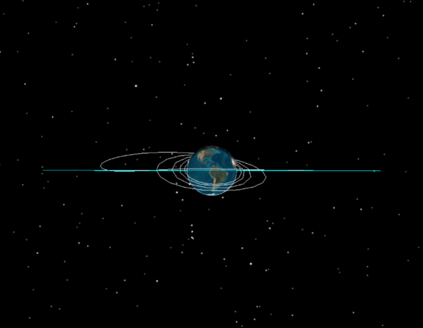
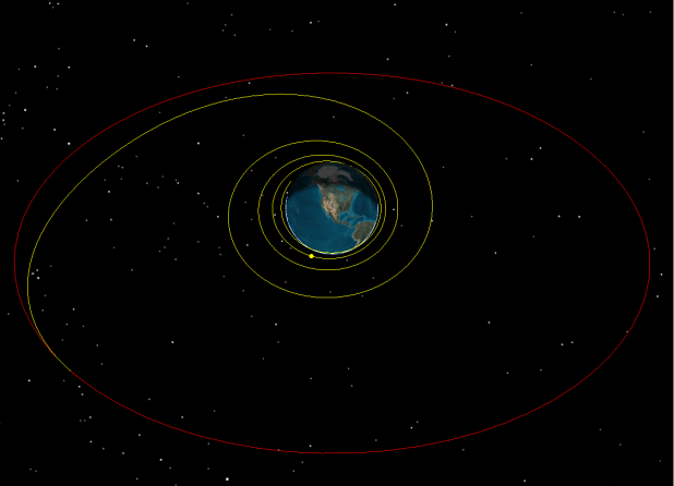
Optimal_Finite satellite propagated into GEO
Note the coarse trajectory drawn by the maneuver. The trajectory is currently showing the node points and lines connecting them.
Exporting the nodes
Once you have the final analysis, you can export the data from the Maneuver segment's Steering/Nodes tab as a Collocation Node file (*.nod). A
- Return to Optimal_Finite's () Properties ().
- Select Maneuver () in the MCS.
- Select the Steering/Nodes tab.
- Examine the Azimuth and Elevation columns.
- Click in the Export panel to save your analysis.
- Enter Low_Thrust_Optimization_GEO_Spiral_120 in the File name field when the Export Nodes dialog box opens.
- Click to confirm your selection and to close the Export Nodes dialog box.
- Save () your scenario.
The values should now reflect the changing direction of thrust.
The default save location is in your scenario folder.
Once you export the optimizer output as a node file, you can subsequently use it for seeding purposes.
Smoothing the trajectory by Running current nodes
You can update and re-run the MCS to produce a smoother result by selecting the Run Mode to Run current nodes. After attempting maneuver optimization, when you select the Run Mode to Run current nodes, running the MCS propagates the vehicle with the states returned from the optimizer and, if successful, the optimal maneuver pointing history.
- Select the Solver tab.
- Open the Run Mode drop-down list in the Problem Execution panel.
- Select Run current nodes.
Running the MCS for the Optimal Finite Maneuver
With your MCS configured, run the entire MCS.
- Click Run Entire Mission Control Sequence () on the MCS toolbar.
- Click to confirm your change and to close the Properties Browser.
- Bring the 3D Graphics window to the front to view the results.
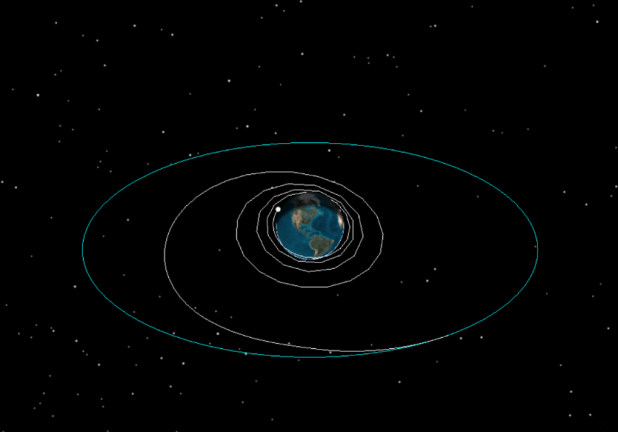
Initial coarse trajectory showing node points
Re-run smoothed trajectory
Using an Initial Guess file
In the previous analysis, you used the Finite Maneuver as the initial guess. This time, use the Collocation Node file you exported earlier for a your Initial Guess. An
Creating a new satellite
For the purposes of this tutorial, copy the existing Optimal_Finite satellite and rename it. This will reduce the amount of time and effort needed to configure the satellite.
- Copy () Optimal_Finite () in the Object Browser.
- Paste () Optimal_Finite () into the Object Browser.
- Rename Optimal_Finite 1 () OptFinite_File.
- Clear the check box for Optimal_Finite () in the Object Browser.
You do not need to re-run the MCS to create the Finite Maneuver if you are using an Initial Guess file.
Updating the Maneuver segment's color
Update the Maneuver segment's color.
- Open OptFinite_File's () Properties ().
- Select Maneuver () in the MCS when the Properties Browser opens.
- Click Segment Properties () on the MCS toolbar.
- Open the Color drop-down list when the Edit Segment dialog box opens.
- Select a color that's different from Optimal_Finite's () Maneuver () and Propagate () segments.
- Click to confirm your change and to keep the Properties Browser open.
Loading the Initial Guess node file
The Initial Guess node file contains the ephemeris data for a satellite maneuver. Using a node file enables you to save different forms of converged solutions that can vary:
- the force model
- the number of nodes
- the control strategy (angles vs. unit vectors)
Using a node file allows you to take data from another tool, format it appropriately, and load it into Astrogator. It also provides a mechanism to solve the problem in stages using a previous solution as an initial guess for a more complex force model. Use the node file you exported earlier in this lesson for your initial guess.
- Select the Solver tab.
- Click the Initial Guess File ellipsis () in the Problem Setup panel.
- Navigate to the location of the Collocated Node file when the Select File dialog box opens.
- Select Low_Thrust_Optimization_GEO_Spiral_120.nod.
- Click to confirm your selection and to close the Select File dialog box.
- Click to confirm your change and to keep the Properties Browser open.
Seeding the initial guess
In this step, you will seed the data from the file into your calculation. This provides the Optimal Finite Maneuver with starting values to compute the optimal low thrust maneuver.
- Select the Seed from - Initial Guess File option in the Problem Setup panel.
- Click .
- Note the Node Status has been updated to note 120 nodes seeded from file.
- Click to confirm your changes and to keep the Properties Browser open.
For more information on seeding an Optimal Finite Maneuver from a file, refer to the Astrogator
Reviewing the Boundary and Path conditions
Review the Boundary and Path conditions to confirm they are the same as those you used when you seeded the Optimal Finite Maneuver from a Finite Maneuver.
- Click .
- Review the explicit values when the Initial Boundary Conditions dialog box opens.
- Click to close the Initial Boundary Conditions dialog box without making any changes.
- Click .
- Confirm the following values are set in the Set Explicitly panel:
- Click to close the Final Boundary Conditions dialog box without making any changes.
- Click .
- Confirm the following values are set in the State Element Variables dialog box:
- Click to close the Path Boundaries for Variables dialog box without making any changes.
| Lower Bound | Variable | Upper Bound |
|---|---|---|
| 42000 km | a | 42000 km |
| 0 | h | 0 |
| 0 | k | 0 |
| 0 | p | 0 |
| 0 | q | 0 |
| 0 deg | L | 1800 deg |
| Tf - 7200 sec | Final Time | Tf + 7200 sec |
| Lower Bound | Variable | Upper Bound |
|---|---|---|
| 6000 km | a | 65000 km |
| -0.9 | h | 0.9 |
| -0.9 | k | 0.9 |
| -0.9 | p | 0.9 |
| -0.9 | q | 0.9 |
| 140 deg | L | 1800 deg |
Setting the Run Mode to Optimize via direct transcription
Set the Run Mode to Optimize via direct transcription to use the optimizer.
- Open the Run Mode drop-down list in the Problem Execution panel.
- Select Optimize via direct transcription.
- Click to confirm your change and to keep the Properties Browser open.
Confirming the Engine model component
Before you run this model, confirm that you are using the correct Engine Model component.
- Select the Engine tab.
- Confirm the Engine Model is set to My Engine in the Propulsion Type panel.
- Confirm the Pressure mode is set to Pressure-Regulated.
- Confirm that the Thrust Efficiency is 1.
- Confirm that the Thrust is set to Affects Accel Only.
Updating the Propagate segment's color
Change the Propagate segment's color.
- Select Propagate () in the MCS.
- Click Segment Properties () on the MCS toolbar.
- Open the Color drop-down list when the Edit Segment dialog box opens.
- Select a color that's different from Optimal_Finite's () Maneuver () and Propagate () segments.
- Click to confirm your change and to keep the Properties Browser open.
- Save () your scenario.
Running the MCS for the Optimal Finite Maneuver
With your MCS configured run the entire MCS.
- Click Run Entire Mission Control Sequence () on the MCS toolbar.
- Review the details in the Optimal Finite Maneuver: optimizer output console window.
- Close the Optimal Finite Maneuver: optimizer output console window when you are finished.
- Bring the 3D Graphics window to the front to view the results.
As before, the Optimal Finite Maneuver: optimizer output console window appears and steps through the analysis.
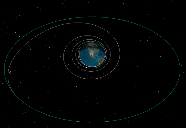
OptFinite_File satellite propagated into GEO
Smoothing the trajectory by Running current nodes
Update the coarse trajectory drawn by the maneuver by setting the Run Mode to Run current nodes.
- Return to OptFinite_File's () Properties ().
- Select Maneuver () in the MCS.
- Select the Solver tab.
- Open the Run Mode drop-down list in the Problem Execution panel.
- Select Run current nodes.
Running the MCS for the Optimal Finite Maneuver
With your MCS configured run the entire MCS.
- Click Run Entire Mission Control Sequence () on the MCS toolbar.
- Click to confirm your changes and to close the Properties Browser.
- Bring the 3D Graphics window to the front to view the results.
trajectory RE-run from current nodes
If you enable the display of Optimal_Finite (![]() ) in the Object Browser, you can see the propagated orbits are the same, which is expected. By using the Initial Guess file, however, you were able to perform the optimization calculations much more quickly.
) in the Object Browser, you can see the propagated orbits are the same, which is expected. By using the Initial Guess file, however, you were able to perform the optimization calculations much more quickly.
Analyzing the mission data
Now that you have the final trajectories for the spacecraft, you can generate data about the mission.
Creating a custom Graph style
Create a custom graph style to plot the angle history of the OptFinite_File satellite.
- Bring the Report & Graph Manager () to the front.
- Select OptFinite_File () in the Object Type list.
- Select the MyStyles () folder in the Styles panel list.
- Click Create new graph style (
 ) on the Styles toolbar.
 - Rename the new graph Angle History.
- Select the Enter key.
Selecting the data providers
Next, choose the data providers for your custom graph.
- Select the Content page when the Properties Browser opens.
- Expand () the Vector Choose Axes () data provider.
- Expand () the TotalThrust () data provider group.
- Move (
 ) the following data provider elements to the Y Axis list:
 - RightAscension (
 )
) - Declination ()
- Click to confirm your selections and to close the Properties Browser.
Generating the Angle History graph
Generate the graph based on the ICR axes.
- Ensure AngleHistory (
 ) is selected in the Styles list.
 - Click .
- Select OptFinite_File () in the Filter by: All STK Objects list when the Select Axes dialog box opens.
- Select ICR (
 ) in the Axes for: OptFinite_File list.
 - Click to confirm your selections and to generate the graph.
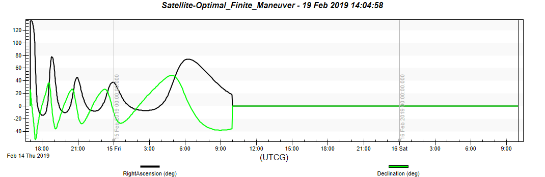
You can see how the direction of thrust changes over the course of the mission until its last segment. In the last segment, the final orbit is propagated.
Generating a Maneuver Summary report for comparison
Compare the results of your Optimal Finite Maneuver to your initial Finite Maneuver by generating another Maneuver Summary report.
- Bring the Report & Graph Manager () to the front.
- Expand () the Installed Styles () folder in the Styles panel list.
- Select Maneuver Summary ().
- Click .
- Take note the Duration of the burn as well as the total Delta V and Fuel Used.
- Compare these values to the Maneuver Summary report you created earlier.
You can see your optimized maneuver had a shorter duration and a lesser Delta-V, thus requiring less fuel.
Saving your work
Clean up and close out your scenario.
- Close any open graphs, reports, properties, and the Report & Graph Manager.
- Save () your work.
Summary
You began by setting up a basic Astrogator satellite. After creating a custom low-thrust engine model, you configured a basic Mission Control Sequence utilizing a Finite Maneuver segment. You then used this Finite Maneuver as an initial guess for an Optimal Finite Maneuver segment, which used a SNOPT search profile to find a feasible, optimum solution. You exported the solution as a Collocated Node file, then, after running the current nodes to smooth the satellite's trajectory, imported the file as an initial guess for another Optimal Finite Maneuver. Finally, you created a custom graph to view the changes in the thrust axes over time to help visualize the optimal low-thrust maneuver and generated Maneuver Summary reports to quantify the differences between your initial Finite Maneuver and your final Optimal Finite Maneuver.