State Transition Matrix (STM) Primer
STK Premium (Space), or STK Enterprise. You can obtain the necessary licenses for this training by contacting AGI Support at support@agi.com or 1-800-924-7244.
The results of the tutorial may vary depending on the user settings and data enabled (online operations, terrain server, dynamic Earth data, etc.). It is acceptable to have different results.
This lesson requires STK 12.4 or newer to complete it in its entirety. It includes new features introduced in STK 12.4.
Throughout our documentation we take some lattitude when referring to the "state transition matrix" depending on the context. The "state transition matrix" technically refers to a matrix that maps an entire state vector in a linear system from some time forward or backward. This results in a new state vector at a new time.
For a nonlinear system, we construct a similar transition matrix that maps small variations ("errors," "perturbations") from a state at a start time along a reference path forward or backward in time. This results in a deviation from the reference at the end time.
This matrix is often denoted the "state transition matrix" or "error state transition matrix," particularly in the context of orbit estimation. In the context of trajectory design, the "error" modifier is frequently dropped since it is uncommon for the dynamical system under analysis to be linear.
STK capabilities covered
This lesson covers the following STK Capabilities:
- STK Pro
- Astrogator
- Analysis Workbench
Problem statement
If you want to launch missions in Earth-Moon space, you need to understand the stability characteristic of a satellite's orbit in that regime. By understanding the stability information, you have a hint into the localized linear motion that could be extended to the underlying nonlinear solution.
Solution
With STK 12.4 and newer, you have the State Transition Matrix (STM) solutions at your fingertips. In this State Transition Matrix (STM) Primer, you will calculate the eigenvalues and eigenvectors for your orbits using STK. You will also examine an application of the Lambert Search Profile, which connects your satellite's initial orbit into a manifold arc that takes it into its final halo orbit.
What you will learn
Upon completion of this tutorial, you will be able to:
- Generate the STM results.
- Understand the significance of the resulting eigenvalues.
- Connect the trajectory arc with the manifold.
Video Guidance
Watch the following video. Then follow the steps below, which incorporate the systems and missions you work on (sample inputs provided).
Please note, the video refers to files accessed from the STK Data Federate (SDF). Any files previously located on the SDF are now available from agi.com. Please follow the written steps in this tutorial to download the files.
Downloading the required starter scenario
You need to download a starter scenario which contains the various halo orbits you will use in this lesson. The scenario is saved as a visual data file (VDF).
- Download the zipped folder here: https://support.agi.com/download/?type=training&dir=sdf/help&file=EarthLunaStableHalos.zip
If you are not already logged in, you will be prompted to log in to agi.com to download the file. If you do not have an agi.com account, you will need to create one. The user approval process can take up to three (3) business days. Please contact support@agi.com if you need access sooner.
- Navigate to the downloaded folder.
- Right-click on EarthLunaStableHalos.zip.
- Select Extract All...
- Set the Files will be extracted to this folder: path to the location of your choice. The default path is C:\Users\<username>\Downloads\EarthLunaStableHalos).
- Click .
- Go to the chosen folder.
- The EarthLunaStableHalos.vdf will be in the extracted folder.
Opening the starter scenario
Open the downloaded scenario.
- Launch the STK (
 ) application.
 - Click Open a Scenario (
 ) in the Welcome to STK dialog box.
 - Browse to location of your extracted VDF file.
- Select EarthLunaStableHalos.vdf.
- Click .
Saving a VDF file as a Scenario file
Save your scenario in an appropriate location for your work.
- Open the File menu.
- Select Save As...
- Select the STK User folder in the navigation pane when the Save As dialog box opens.
- Click the New Folder option in the selector bar.
- Name the New folder EarthLunaStableHalos.
- Select the EarthLunaStableHalos folder.
- Click .
- Select Scenario Files (*.sc) as the Save as type.
- Enter EarthLunaStableHalos.sc as the File name.
- Click .
Save Often!
Understanding the state transition matrix (STM)
Now that the scenario is open, you will examine the 3D Graphics windows and the various halo orbits. Before diving into the properties, let's discuss the state transition matrix (STM). The STM captures the effects of small changes to an initial state as they propagate along a reference path to some terminal state. This matrix is produced by taking a first-order Taylor series truncation of the underlying system equations of motion and numerically integrating the associated variational equations. It is often represented by where
where is the initial time and
 is the time at which the STM is being calculated. The propagation of an initial perturbation is expressed notationally as
This matrix, in an astrodynamics context, is a 6x6 matrix capturing the effects of initial perturbations on each of the position and velocity components of the state with respect to each of the final position and velocity components. For example, a particular component of the STM may yield the effects of an initial perturbation to the y component of velocity on the final z component of position thus:

The STM can be propagated with a trajectory in STK's Astrogator capability by adding the STM propagation function to the propagator. For this tutorial, you will generally use a circular restricted three-body problem (CR3BP) propagator with the STM included to take advantage of the underlying autonomous dynamical system and its associated mathematical properties.
After computing the STM, a frequent activity is to compute its associated eigenvalues and eigenvectors to learn about the stability properties of the associated propagated trajectory. If that trajectory happens to be a periodic orbit like a libration point orbit about one of the libration points in a three-body system, you will compute the monodromy matrix, M, which is the STM after one period, T, of the orbit.
The eigenvalues and eigenvectors of this matrix give us insight into the linear stability of the orbit. Typically, in an orbit such as an L1 halo orbit the eigenvalue spectrum, λ , takes the following form:

The two eigenvalues that are unitary correspond to the periodic orbital motion and the existence of nearby solutions belonging to a continuous family of similar orbits. The complex eigenvalues indicate the propensity for circulation about the orbit and the real eigenvalues, one larger than magnitude one accompanied by its inverse, indicate the presence of stable and unstable modes of the orbit – the possibility for trajectories to asymptotically flow into or away from the orbit. In some cases, the eigenvalue structure is comprised of two unitary and four complex eigenvalues. In these cases, such an orbit does not possess stable or unstable modes and is considered fully stable in the linear sense.
Understanding Halo orbits
In the following figure, a representative L1 halo orbit within a family of such orbits is depicted. General orbits in this family are colored in blue and pink. A region of stable orbits is indicated by green representative orbits. You will take a closer look at the yellow orbit seen in Figure 1 later.
- Maximize the Halos 3D Graphics window in the STK scenario.
- Examine the different orbits.
- Rotate the view to see the perspectives below.
Figure 1 - L1 halo orbits looking back toward the Earth from the Moon (Luna)
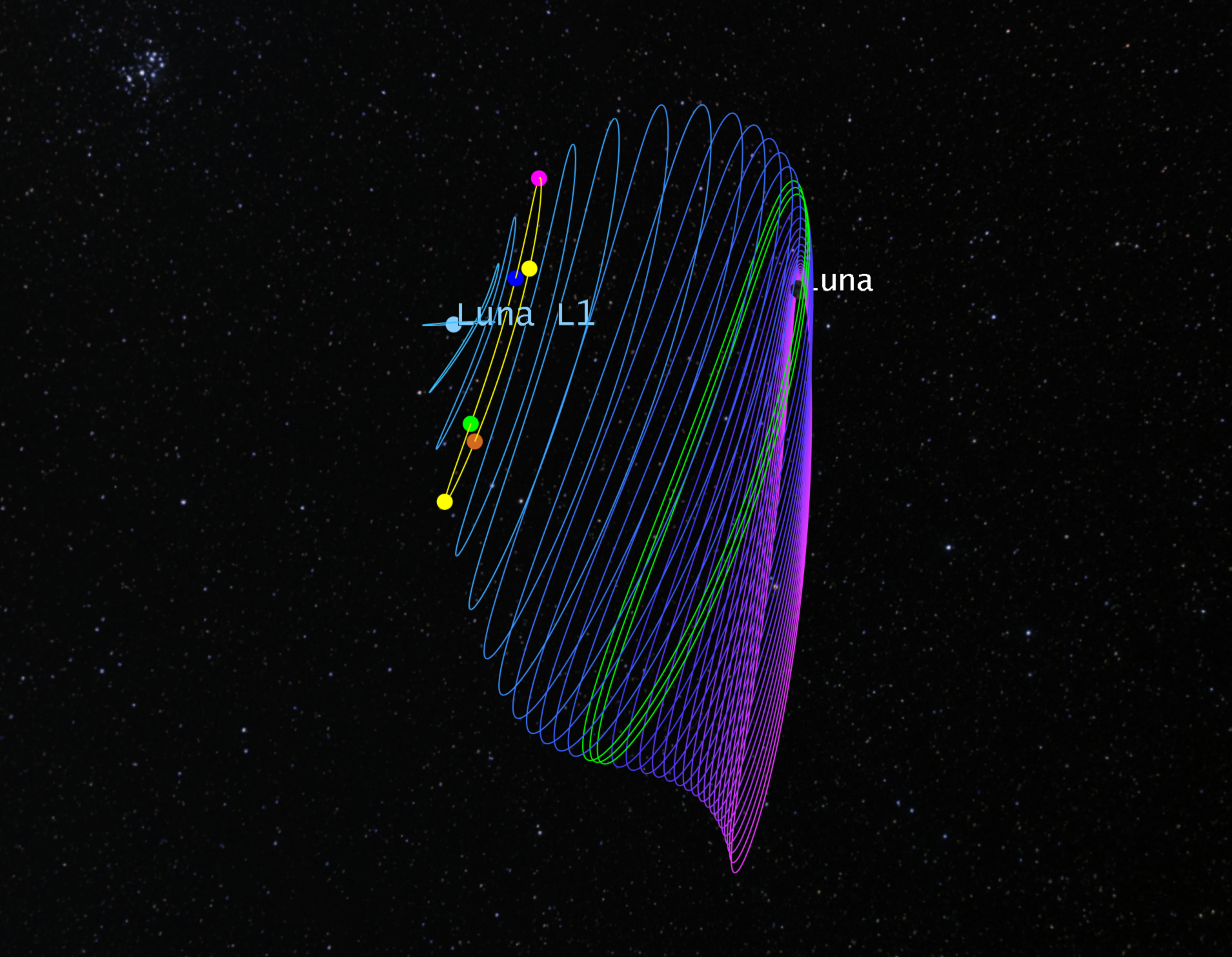
Figure 2 - Side view of Figure 1
Examine a green orbit first before diving into the rest of your analysis.
Examining a satellite orbit with complex eigenvalues
You will first examine the STM of a satellite with complex eigenvalues. Before doing that, you will modify the propagate segments and run the MCS. Please keep the work flow in mind as you generate the STM for your other halo orbits.
- Open Halo028g's (
 ) properties (
 ).
). - Select the Basic - Orbit page.
- Select the Propagate (
 ) segment in the MCS.
 - Right-click on the Propagate (
 ) segment.
 - Select Properties... from the menu.
- Change the Coordinate System to EarthLunaBarycentered. This will change the coordinate system for the reporting frame.
- Click .
Running the Mission Control Sequence (MCS)
Once the propagate segment's coordinate system is updated, run the Mission Control Sequence to calculate the trajectory of the spacecraft. This will calculate your results, including the Jacobi constant.
- Click Run Entire Mission Control Sequence (
 ) in the MCS toolbar.
 - Watch the MCS in the 3D Graphics window. This analysis was already run, so you may not see any changes in your graphics display.
Generating an MCS propagate summary report
Generate an MCS propagate summary report and analyze the Eigenvalues.
- Select the Propagate () segment in the MCS.
- Click the Summary (
 ) icon in the MSC toolbar.
 - Scroll to the end of the report.
- Analyze STM Eigenvalues. Since this is a periodic orbit, you should see a pair of values that are 1 (or very close to 1). The values come in pairs, and all the eigenvalues are complex. If all the values are complex and you have two 1 values, that means unstable or stable modes do not exist for the orbit.
- Close (
 ) the Report.
 - Close the properties window.
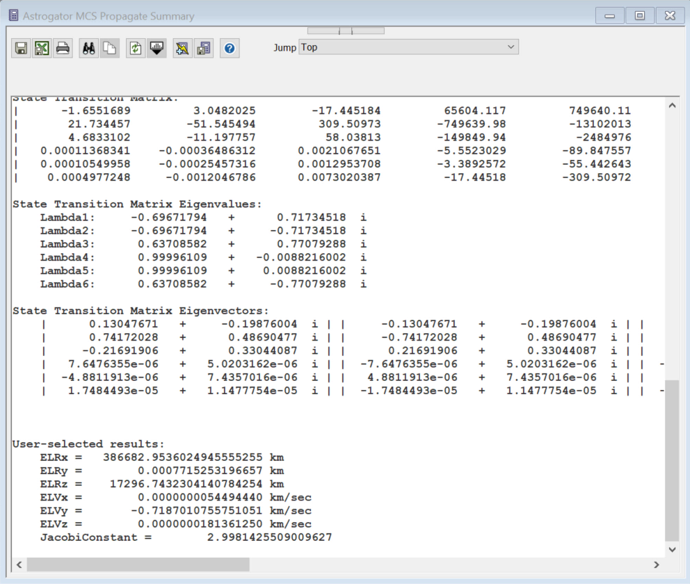
Figure 3: MCS Propagate Summary report for Halo028g.
Next, examine the yellow orbit, which does have stable and unstable modes.
Examining stable and unstable modes
When an orbit has stable and unstable modes, nonlinear flow can be isolated that approaches or departs the orbit on structures called stable and unstable manifolds, respectively. Look at that yellow orbit specifically.
- Open Halo007y's () properties (
 ).
). - Select the Basic - Orbit page.
- Select the Propagate () segment in the MCS.
- Right-click and select Properties from the menu.
- Confirm or change the Coordinate System to EarthLunaBarycentered. This will change the coordinate system for the reporting frame.
- Click .
Running the MCS
Once the propagate segment's coordinate system is updated, run the MCS to calculate the trajectory of the spacecraft.
- Click Run Entire Mission Control Sequence (
 ) in the MCS toolbar.
 - Examine the Halo007 3D Graphics window in the STK scenario. You should see the below perspective.
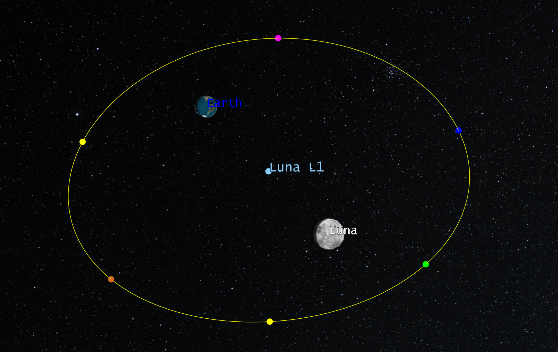
Figure 4 - L1 halo orbit viewed along the line from Luna back toward the Earth
If you compute the eigenvalues and eigenvectors of the monodromy matrix at a few points around the orbit including the initial point (magenta in the image above), you can determine the stability properties of this orbit and directions that will lie along stable and unstable manifolds associated with your representative points. The yellow orbit above is characteristic of the monodromy matrix , associated eigenvalues, and its first two eigenvectors reported in the subsequent section. These values are computed in the Earth-Luna rotating frame.
Generating an MCS propagate summary report
Examine the behavior of this halo orbit.
- Select the Propagate () segment in the MCS.
- Click the Summary () icon in the MSC toolbar.
- Scroll to the end of the report.
- Notice that the results demonstrate a hyperbolically stable orbit, meaning there is a stable and an unstable mode.

Figure 5 – STM after one period (M), eigenvalues and eigenvectors
Lambda1 indicates an unstable mode (large real number), and Lambda 2 indicates a stable mode (small real number). The respective eigenvectors, unstable and stable, are shown below with the third eigenvector extending beyond the snapshot. The third and fourth eigenvalues are very close to 1 and correspond to orbital motion and the presence of nearby orbits in the family. The remaining two eigenvectors correspond to portions of the center manifold and indicate that circulation about the orbit exists.
If you find the stable eigenvectors for each of the representative points in Figure 4, you can perturb motion in their associated direction and propagate backward in time to produce portions of the stable manifold that flows into the orbit (in forward time).
Each trajectory is an arc on the surface of the manifold. If 100 or even 1000 more trajectories were found and perturbed, you would see more of the entire "tube". Given a certain energy level, there are some regions where you can go into the orbit without a maneuver. Being on any point on the surface of the tube means the satellite will flow into the orbit. If you are inside of the tube, you will transit into the lunar region without a maneuver. Objects outside of it will remain in the region associate with the Earth, unless there is a maneuver.
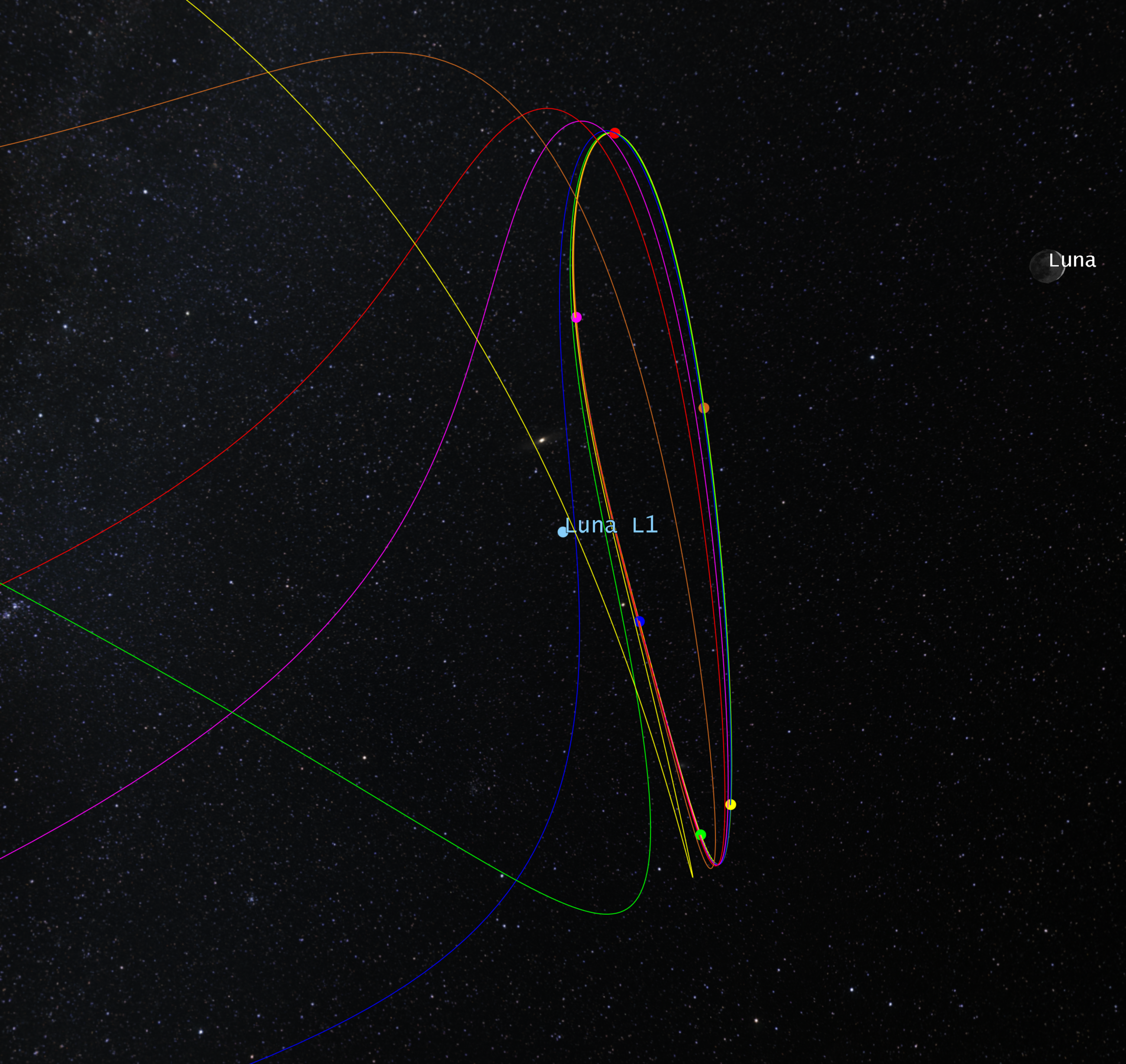
Figure 6 - Manifold arcs winding into the halo orbit
Examining a Lambert arc
A more wide-angle view shows these manifolds arcs propagated backward in time until their third associated periapsis passages with respect to the Earth. It also includes a Lambert arc departing a LEO and connecting to a selected manifold arc (red). You will now dive into its properties.
- Open ALeoToMan's () properties ().
- Select the Basic - Orbit page.
- Select the Target sequence in the MCS.
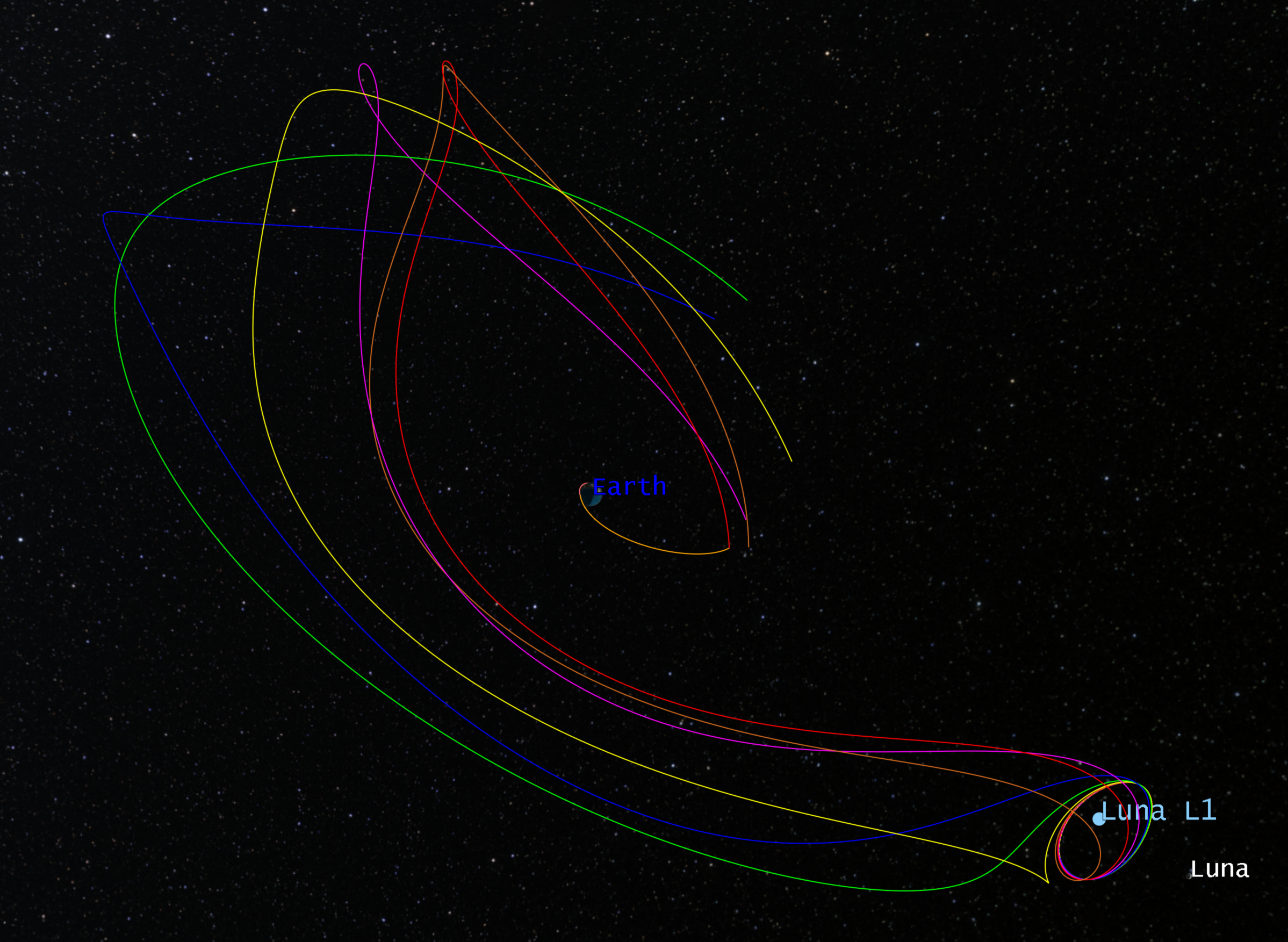
Figure 7 - Lambert arc from LEO connecting into a manifold arc flowing into the L1 halo orbit
Examining the target sequence
Examine the strategy used to achieve the solution. In the target sequence, you will examine the four profiles. The first is a Lambert Search Profile. The Lambert Search Profile always solves using a two-body model. The next two profiles are Change Propagators. While the Change Propagator profile approach is a common Astrogator work flow, it is not actually required in this case, as you could set the propagator to three-body. This work flow is included for demonstration. Finally, you will examine the Differential Corrector to see how to target the final solution.
- Open the Lambert Search Profile's properties ().
- You can use the Lambert Search to go from an initial position to a final state associated with the manifold. In this case, you have taken the position of the satellite at the end of the manifold (the third periapsis point) in the Earth Inertial state and plugged it in.
- Click without making any changes.
- Open the Change Propagator's properties ().
- Take a look at how you are changing the propagator to a higher fidelity model. You initially solved the two-body problem; by changing the propagator, you are transitioning the solution from two-body to three-body.
- The settings for Change Propagator1 are the same as the previous segment and are done for the same stated reason.
- Click without making any changes.
- Open the Differential Corrector's properties ().
- You are targeting the position and velocity components at the end of the sequence. That's because you want to target where the satellite will be on the manifold, which you can determine using your two maneuvers and Lambert duration stopping conditions.
- Click without making any changes.
Running the MCS
Once you have examined the Target Sequence, run the MCS to calculate the trajectory of the spacecraft.
- Click Run Entire Mission Control Sequence () in the MCS toolbar.
- Examine the Inertial Graphics window in the STK scenario. You should see the below perspective.
You see the same solution connecting LEO to the L1 halo orbit, but from the perspective of an inertial frame. The interface point between the red manifold arc and the yellow halo orbit propagation occurs at the epoch (i.e., relative geometry between the Earth and Luna) shown in the figure.
You developed this mission in the rotating frame and are demonstrating the behavior an observer would see in the inertial frame.
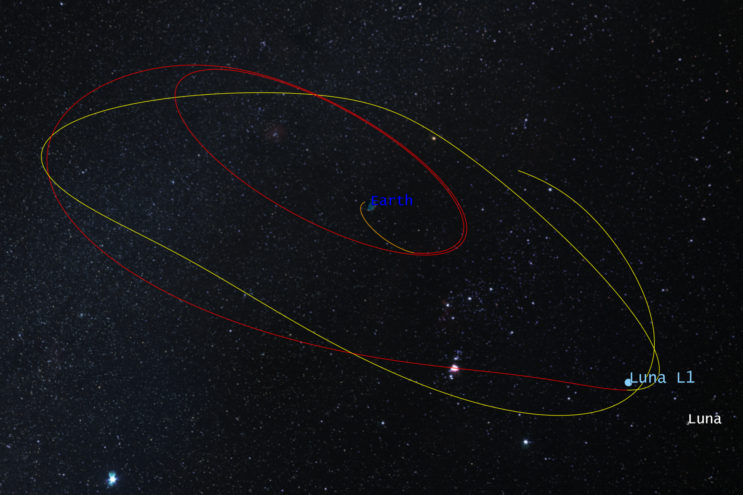
Figure 8 - Inertial view of the Lambert arc, red manifold and halo orbit propagation from Figure 7
Saving your work
- Reset (
 ) the scenario and close any reports, graphs or tools that are still open.
 - Save (
 ) your work.
Conclusion
In this lesson, you explored a prebuilt scenario. The scenario modeled a few halo orbits around Earth-Moon L1. You examined one with complex eigenvalues and then one with real eigenvalues, the latter demonstrating stable and unstable modes. You examined the Lambert Search profile that enabled you to target the surface of the manifold and take your satellite into its final halo orbit around the libration point. You demonstrated with your change propagate profiles and your differential corrector how to take the two-body solution to a final, higher fidelity three-body solution.
On your own
You examined a few halo orbits in this lesson. On your own, run the MCS and examine the STM, eigenvalues, and eigenvectors of some of the other halo orbits.