STK Premium (Air) or STK Enterprise
You can obtain the necessary licenses for this tutorial by contacting AGI Support at support@agi.com or 1-800-924-7244.
Required product install: The Ansys ModelCenter® model-based systems engineering software and the STK Plugin for ModelCenter are required to complete this tutorial. The ModelCenter software is available through the Ansys Universal Installer and the STK Plugin for ModelCenter is included with the STK Premium installation. Contact AGI support for installation help.
ModelCenter installation prerequisites: The ModelCenter software installs the current version of Java and Python supported by Ansys, but you can also use your own versions. See the Installation instructions in the ModelCenter Installation Guide and Supported Versions documentation for more information. Contact AGI support for help with installation.
This tutorial was written using version 2026 R1 of the Ansys ModelCenter® model-based systems engineering software. Refer to the ModelCenter Supported Versions page in the ModelCenter Installation Guide and Supported Versions documentation for compatibility information.
The results of the tutorial may vary depending on the user settings and data enabled (online operations, terrain server, dynamic Earth data, etc.). It is acceptable to have different results.
Capabilities covered
This lesson covers the following capabilities of the Ansys Systems Tool Kit® (STK®) digital mission engineering software:
- STK Pro
- Aviator
- STK Analyzer
Problem statement
Aircrew and mission planners require a quick way to determine how wind and airspeed will affect an aircraft's fuel consumption for a planned flight route. A C-17 Globemaster III cargo aircraft will fly from Joint Base Pearl Harbor–Hickam in Hawaii to Travis Air Force Base in California. Though the aircraft has a fuel capacity of 239,655 pounds of JP-8 jet fuel, it has approximately 181,100 pounds of fuel on board. The aircraft will fly at an altitude of 28,000 feet mean sea level (MSL). Winds are forecast to be at 30 miles per hour. The winds could blow from varying directions due to storms along the way. Additionally, the aircraft has a range of airspeeds at which it can fly; the speeds have differential rates of fuel consumption and can be categorized in terms of maximum endurance, maximum range, and so on. You want to determine the amount of fuel consumed based on the worst-case scenario as well as the best cruising speed under the circumstances.
Solution
Use the STK software's Aviator capability and the Analyzer capability, which is part of the Ansys ModelCenter® model-based systems engineering software, to determine how wind speed, wind direction and the aircraft's airspeed will affect its fuel consumption over the course of the flight.
What you will learn
Upon completion of this tutorial, you will understand how to:
- Insert an aircraft from the online Aircraft database
- Update an Aviator mission wind model
- Update an aircraft model's speed
- Use the Aviator capability with the STK Plugin for ModelCenter
Creating a new scenario
First, you must create a new scenario, then build from there.
- Launch the STK application (
 ).
). - Click
 Create a Scenario in the Welcome to STK dialog box.
 - Enter the following in the New Scenario Wizard:
- Click when you finish.
- Click Save (
 ) when the scenario loads.
 - Verify the scenario name and location in the Save As window.
- Click .
| Option | Value |
|---|---|
| Name | Aviator_ModelCenter |
| Location | Default |
| Start | Default / Set the time to 20:00:00.000 UTCG |
| Stop | + 6 hrs |
The STK software creates a folder with the same name as your scenario for you.
Save () often during this tutorial!
Inserting Place objects to be used as Aviator waypoints
The C-17 Globemaster III aircraft will fly from Joint Base Pearl Harbor–Hickam to Travis Air Force Base. You can model these locations using two
Inserting Joint Base Pearl Harbor-Hickam
Start by inserting Joint Base Pearl Harbor-Hickam.
- Bring the Insert STK Objects tool (
 ) to the front.
 - Select Place (
 ) in the Select An Object To Be Inserted list.
 - Select Define Properties (
 ) in the Select A Method list.
 - Click .
- Select the Basic - Position page when the Properties Browser opens.
- Enter the following values in the Position panel:
- Click to confirm your changes and to close the Properties Browser.
- Right-click on Place1 () in the Object Browser.
- Select Rename in the shortcut menu.
- Rename Place1 () Hickam.
| Option | Value |
|---|---|
| Latitude | 21.32 deg |
| Longitude | -157.923 deg |
Inserting Travis Air Force Base
Next, insert Travis Air Force Base.
- Bring the Insert STK Objects tool () to the front.
- Insert a Place () object using the Define Properties () method.
- Select the Basic - Position page when the Properties Browser opens.
- Enter the following values in the Position panel:
- Click to confirm your changes and to close the Properties Browser.
- Rename Place2 () Travis.
| Option | Value |
|---|---|
| Latitude | 38.26 deg |
| Longitude | -121.93 deg |
Inserting an Aircraft object from the Standard Object Database
You can use the Standard Object Database tool to search for and
- Bring the Insert STK Objects tool () to the front.
- Insert an Aircraft (
 ) object using the From Standard Object Database (
 ) method.
 - Enter Globemaster in the Name field when the Search Standard Object Data dialog box opens.
- Click .
- Select C-17_Globemaster_III in the Results list.
- Click .
- Click to close the Search Standard Object Data dialog box.
In addition to the name, you can search aircraft by many criteria, including manufacturer, keywords, and designations like patrol, drone, and so on.
All aircraft that meet your search criteria are listed, along with their manufacturer, maximum True Airspeed, Operational Range, Endurance, Ceiling Altitude, and Designation.
If you are working in an environment without internet connectivity, you can create a Aviator aircraft and use a copy of the installed Basic Airliner aircraft model, as described in the
Updating the aircraft's properties
You will make a few modifications to C-17_Globemaster_III's properties so that you can analyze them using the ModelCenter application.
Opening and reviewing the aircraft's properties
Take a look at C-17_Globemaster_III's properties.
- Right-click on C-17_Globemaster_III () in the Object Browser.
- Select Properties () in the shortcut menu.
- Select the Basic - Route page when the Properties Browser opens.
- Note that Aviator is already selected as the propagator.
- Note that C-17 Globemaster III is selected in the Initial Aircraft Setup panel.
With Aviator, the aircraft's route is modeled by a sequence of curves parameterized by well-known performance characteristics of aircraft, including cruise airspeed, climb rate, roll rate, and bank angle.
In Aviator, the
Optimizing STK for Aviator
Aviator performs best in the 3D Graphics window when the surface reference of the globe is set to Mean Sea Level (MSL) instead of the default reference of WGS84. Likewise, setting the animation mode to X Real Time allows for smoother animation and better data display performance.
- Click to confirm your aircraft configuration and to keep the Properties Browser open.
- Read the information in the Flight Path Warning dialog box that appears.
- Click to set the scenario globe reference to MSL and the Animation mode to X Real Time.
- Click to close the Fight Path Warning dialog box.
Adjusting the Mission Wind Model
Use the
- Click Mission Wind Model (
 ) on the Initial Aircraft Setup toolbar.
 - Note that the Model Type defaults to Constant Bearing/Speed when the Mission_Acft (UI) wind/atmosphere model dialog box opens.
- Enter 30 nm/hr in the Wind Speed field.
- Click to confirm your change and to close the Mission_Acft (UI) wind/atmosphere model dialog box.
- Click to confirm your changes and to keep the Properties Browser open.
Building the phases of flight with sites and procedures
An aircraft using Aviator is defined by the type of aircraft and by the mission it performs. A mission is a sequence of procedures that utilize aircraft performance models to define the vehicle's route and flight characteristics.
Selecting Hickam as your first site
Each phase is composed of procedures and sites. A
- Note that Phase1 (
 ) is the only phase listed in the mission list.
 - Click Insert Procedure After (
 ) on the Procedures and Sites toolbar.
 - Select STK Static Object (
 ) in the Select Site Type list when the Site Properties dialog box opens.
 - Enter Hickam in the Name field.
- Select Hickam () in the Link To list.
- Click .
The mission list in the mission window provides an overview of the mission by listing each of the mission phases and the procedures within them in the order in which they will be executed.
An STK
Selecting a Basic Point to Point procedure
A Basic Point to Point procedure is a basic traverse between two waypoints. That is, it smoothly accelerates/decelerates under a constant climb/descent to arrive at the specified speed, altitude, and heading The direction that the aircraft is pointing.. Using basic point to point, the aircraft uses the
- Select Basic Point to Point (
 ) in the Select Procedure Type list in the Procedure Properties dialog box.
 - Open the Airspeed drop-down list in the Enroute Cruise Airspeed panel.
- Select TAS True Airspeed: the speed that the aircraft is moving relative to the airmass that it is flying in..
True airspeed (TAS) is the actual speed of an aircraft relative to the surrounding air mass.
Reviewing available airspeed types
The Enroute Cruise Airspeed parameters define the airspeed performance characteristics of the aircraft during enroute segments of the procedure. With the exception of Other Airspeed, the actual airspeed will be defined by the currently selected cruise performance model. For your trade studies, you will focus on maximum endurance, maximum range, and maximum performance airspeeds.
- Note that the default enroute cruise airspeed in set to Max Range Airspeed and the airspeed value is 450 nm/hr (nautical miles per hour) true airspeed.
- Open the Airspeed Type drop-down list.
- Select Max Endurance Airspeed.
- Open the Airspeed Type drop-down list.
- Select Max Performance Airspeed.
This airspeed maximizes the distance that the aircraft can fly.
This airspeed maximizes the length of time that the aircraft can remain in flight. The airspeed value is approximately 342 nautical miles per hour true airspeed.
This airspeed optimizes specific flight capabilities. The airspeed value is 475 nautical miles per hour true airspeed.
Based on the aircraft cruise configuration, you will consider an airspeed range from 340 (342 rounded down) to 475 nautical miles per hour in your trade studies.
For this exercise, you are only interested in the fuel consumption during the enroute segment of mission, so you are starting at altitude instead of building a full mission profile with Takeoff, Landing, and other procedures.
Setting the enroute cruise airspeed to use Other Airspeed
Other Airspeed is a constant, manually defined airspeed.
You must use this setting in order to study a range of airspeeds with the ModelCenter application.
- Open the Airspeed Type drop-down list.
- Select Other Airspeed.
- Click to confirm your changes and to close the Procedure Properties dialog box.
- Click to confirm your changes and to keep the Properties Browser open.
Inserting Travis AFB as the second waypoint.
Selecting Travis AFB as the second waypoint.
- Click Insert Procedure After () on the Procedures and Sites toolbar.
- Select STK Static Object () in the Select Site Type list when the Site Properties dialog box opens.
- Enter Travis AFB in the Name field.
- Select Travis () in the Link To list.
- Click .
Selecting a Basic Point to Point procedure
Select a Basic Point to Point procedure.
- Select Basic Point to Point () in the Select Procedure Type list in the Procedure Properties dialog box.
- Open the Airspeed Type drop-down list in the Enroute Cruise Airpseed panel.
- Select Other Airspeed.
- Open the Airspeed drop-down list.
- Select TAS.
- Click to confirm your changes and to close the Procedure Properties dialog box.
- Click to confirm your changes and to close the Properties Browser.
Saving your STK scenario
Before opening the ModelCenter application, save your scenario and close out of the STK application.
- Save () your scenario.
- Close the STK application.
Creating a new ModelCenter project
The Ansys ModelCenter model-based systems engineering software is designed for multidisciplinary analysis and design optimization. It allows you to automate complex workflows, integrate multiple engineering tools, and optimize designs within model-based systems engineering (MBSE) frameworks. By wrapping tools and analysis programs like the STK application and running them in an automated fashion, the ModelCenter software makes the design process more efficient, saves engineering time, and reduces the chances for error in the design process. It implements MBSE processes flexibly; its drag-and-drop graphical user interface can be used to assemble tools into a complete engineering workflow, which can contain branches, loops, logical statements, and more. Your workflow can contain tools that run on any number of different machines and operating systems. Once a repeatable engineering analysis process is created, you can repeatedly execute the process, using parallel computing resources if available. Each execution corresponds to a different set of inputs, which you can use to explore and quantify the performance of your design alternatives in a relatively short time.
- Open the ModelCenter (
 ) application.
 - Click in the Welcome to ModelCenter dialog box.
- Click when the What type of model would you like to create? dialog box opens.
- Navigate to your scenario folder (for example, C:\Users\<username>\Documents\STK_ODTK 13\Aviator_ModelCenter).
- Enter Aviator_ModelCenter in the File name field.
- Ensure the Save as type is set to the ModelCenter Model (Zip) (*.pxcz).
- Click .
A Process is a graphical, flowchart-like workflow that explicitly tells the ModelCenter application what order (and under what conditions) to run each component.
You can learn more about the ModelCenter software
Launching the STK Plugin for ModelCenter
All ModelCenter workflows are built using a simple drag-and-drop scheme for creating a graphical layout of a complex analysis. Process workflows leverage that capability by highlighting "hot spots" for adding and moving components in a workflow. Components encapsulate an analysis or control function. Each component exposes input and output variables and executes a run method to transform inputs into outputs. The
- Note that your empty Process workflow contains a single hot spot, represented by a dashed circle underneath "Drop items here to build the model," in the Analysis View.
- Select favorites (
 ) in the Server Browser at the bottom of the window.
 - Click and drag the STK component (
 ) from the Server Browser onto the hot spot.
 - Select Aviator_ModelCenter.sc when the Open STK Scenario file dialog box opens.
- Click .
This will open the STK scenario and STK Analyzer windows. Please be patient.
The Aviator_ModelCenter scenario file will open in the STK application in the background. If the STK application opens in front of ModelCenter, bring the ModelCenter application window back to the front.
Setting up your analysis with Analyzer
Use the STK Analyzer window to configure the input and output variables available for further analysis with the
Selecting the input variables
Wind bearing and aircraft speed will have an impact on the amount of fuel the aircraft consumes. Add them as your input variables.
- Select C-17_Globemaster_III () in the STK Variables tree.
- Select the General tab in the STK Property Variables panel.
- Expand (
 ) the Propagator (Aviator) (
 ) property in the STK Property Variables tree.
 - Expand () the WindModel (Constant Wind) () property.
- Select WindBearing (
 ).
). - Move (
 ) WindBearing () to the Analyzer Variables list.
 - Expand () the Phase 1 1 () property.
- Expand () the Basic Point to Point 2 () property.
- Select AirSpeed ().
- Move () AirSpeed () to the Analyzer Variables list.
When you select an object in the STK Variables tree, all possible input variable candidates for that object are listed under the General tab and the Active Constraints tab in the STK Property Variables panel.
Basic Point to Point 1 doesn't need to be studied since it's the starting waypoint. The aircraft moves throughout Basic Point to Point 2.
Both AirSpeed and WindBearing are listed as Inputs in the Analyzer Variables list.
Selecting the output variable
The same data providers that are available in the Report & Graph Manager are available in the Data Provider Variables tree.
- Select the Data Providers tab in the Data Provider Variables panel.
- Expand () the Flight Profile By Time (
 ) data provider in the Data Provider Variables tree.
 - Expand () the Fuel Consumed (
 ) data provider element.
 - Select the Max (
 ) statistical function.
 - Move () Max () to the Analyzer Variables list.
- Click to confirm your selections and to close the STK Analyzer window.
Max is now listed under Outputs in the Analyzer Variables list.
This will also close the STK application, which had been running in the background.
Determining the impact of wind bearing on fuel consumed
The first study you will perform varies the wind bearing to determine its effects on how much fuel is used during the mission. The current wind speed of 30 nautical miles per hour will be maintained.
Creating a benchmark
You can quickly analyze your current setup, which will create a benchmark of the output variable values.
- Expand (
 ) all the components in the Component Tree.
 - Note the input variable values in the Component Tree.
- Click Run (
 ) on the Standard toolbar.
 - When completed, note the Max output variable's icon has changed from invalid (
 ) to valid (
 ) and its Value has been computed.
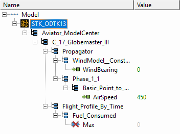
expanded component tree
These are the values imported into ModelCenter from the Aviator_ModelCenter scenario.
The output variable value is based on the default input variables which are a wind bearing of zero (0) degrees and an airspeed of 450 nautical miles per hour.
Using the Parametric Study tool
The Parametric Study tool runs a workflow through a sweep of values for some input variable. You can plot the resulting data to view trends.
- Click Parametric Study (
 ) on the Standard toolbar.
 - Click and drag WindBearing (
 ) from the Component Tree to the Design Variable field when the Parametric Study tool opens.
 - Set the following Design Variable values:
- Click and drag Max () from the Component Tree to the Responses field.
- Click .
| Option | Value |
|---|---|
| starting value | 0 |
| ending value | 360 |
| step size | 30 |
To save time, you are analyzing wind direction in 30-degree increments. On your own, you could use a smaller step size which will increase the number of samples and the amount of time it takes to analyze the wind bearing. You will use large step sizes throughout this analysis to lower the amount of time it takes to complete your trade studies.
Clicking will open the Data Explorer, which is a tool used by Trade Study tools to display data while they are being collected from the STK scenario. While data are being collected, the Data Explorer displays a progress meter, a halt button, and the data. The Table page displays trade study data in a tabular form. It is the default window that is present for all trade studies. Cells are shaded differently depending on the associated variable's state. Input variables are shown with green text, valid values are displayed with black text, invalid values are displayed with gray text, and modified values are displayed with blue text. From the table it is possible to view and edit all values in your trade study and even to add and remove whole runs. The first line shows wind bearing from 0 through 360 degrees. The second line shows the maximum fuel consumed. Remember that the default airspeed is set at the maximum range airspeed of 450 nautical miles per hour.
Creating a 2D Line Plot
Once the trade study is complete and all data have been collected, the Data Explorer toolbar becomes active. The Data Explorer stores values for all variables in a workflow and special variables from the trade study. Some trade study tools will automatically launch a default plot window when the trade study runs. For other plots, you can create them from the Add View menu. For this study, you will create a 2D Line Plot. A 2D Line Plot displays an X-Y plot for variables in your model. Any variable in the workflow can be plotted against any other variable.
- Bring the Data Explorer window to the front when the when the trade study is finished running.
- Click Add View (
 ) on the Data Explorer toolbar.
 - Select 2D Line Plot (
 ) in the drop-down menu.
Setting options for the axes
Use the Axes tab to set options for the axes.
- Click Axes (
 ) in the Plot Options menu on the left-hand side of the 2D Line Plot.
 - Select the Ticks tab.
- Change the Max # value to 30.
- Click anywhere on the plot to close the Plot Options menu.
- Review the 2D Line Plot.
- Hover your cursor over the lowest design point in the plot.
- Click the Open Design View ellipsis in the lower-right corner of the Design Tooltip to open the Design View dialog box.
- When finished, close the Design View.
The Axes tab is used to set options for the plot's axes.
The Ticks tab is used to set the display of ticks along the axes.
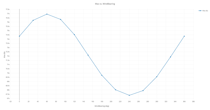
Wind Bearing vs Maximum Fuel Consumed
This will show you information about that point in a Design Tooltip. It's also the wind bearing that is likely a tailwind where the aircraft would consume the least amount of fuel.
This provides more detailed information of the selected design point.
For this flight route, a wind bearing of 60 degrees causes the aircraft to consume the most amount of fuel and a bearing of 240 degrees (the reciprocal heading for 60 degrees) the least amount of fuel.
Closing out your trade study
Close out your trade study for the next section.
- Bring the Data Explorer to the front.
- Close the Data Explorer.
- Click when prompted to close your trade study without saving.
- Leave the Parametric Study tool open.
This will also close all open plots and graphs.
Creating a new Parametric Study
Create a new parametric study to analyze the effects of airspeed on fuel consumption.
- Click and drag AirSpeed () from the Component Tree to the Design Variable field in the Parametric Study tool.
- Set the following Design Variable values:
- Click .
This will replace WindBearing as the Design Variable.
| Option | Value |
|---|---|
| starting value | 340 |
| ending value | 475 |
| step size | 15 |
Reviewing data in the Data Explorer Table
While you can create line plots that are great for presentations or personal choice, you can also obtain the required information directly from the Table page. The Table page of the Data Explorer displays trade study data in a tabular form. It is the default window that is present for all trade studies. Cells are shaded differently depending on the associated variable's state. Input variables are shown with green text, valid values are displayed with black text, invalid values are displayed with gray text, and modified values are displayed with blue text. From the table it is possible to view and edit all values in your trade study and even to add and remove whole runs.
- Bring the Data Explorer to the front when the when the trade study is finished running.
- Examine the results in the Data Explorer Table on the Table Page.
- Right-click on the dependent variable (Model.STK_ODTK13.Aviator_ModelCenter.C_17_Globemaster_III.Flight_Profile_By_Time.Fuel_Consumed.Max) in the AUTO SCROLL LIST in the Data Explorer Table.
- Select Sort Runs in the shortcut menu.
- Select Ascending in the Sort Runs submenu.
- Move the slider at the bottom of the Data Explorer all the way to the left so that you can see the first run.
- Note that the least amount of fuel consumed is at an airspeed of 445 nautical miles per hour.
- Close the Data Explorer.
- Click when prompted to close your trade study without saving.
- Close the Parametric Study tool.

Data Explorer Table
If you recall, 450 nautical miles per hour is the maximum range airspeed. A good assumption is that slower airspeeds consume less fuel. However, that's not the case, as seen in this trade study. Although these values might seem unusual, they're not. The aircraft is configured for maximum range by default. When you changed the Enroute Cruise Airpseed to Other Airspeed, the default was 450 nautical miles per hour true airspeed. That is the optimum maximum range setting based on a lot of other characteristics such as fuel flow, wing design, and so on.
Analyzing the effects of wind bearing and speed together
A Carpet Plot is a means of displaying data dependent on two variables in a format that makes interpretation easier than normal multiple-curve plots. A Carpet Plot can be thought of as a multidimensional Parametric Study. Setting the design variables in a Carpet Plot is similar to using the Parametric Study tool, except you can study two variables simultaneously instead of one.
Creating a new Carpet Plot
You know that wind bearing and airspeed had an impact on fuel consumed. For the purposes of this study, keep the number of steps low for time. However, on your own, you can perform as many runs as you desire.
- Click Carpet Plot (
 ) on the Standard toolbar.
 - Click and drag WindBearing () from the Component Tree to the first Design Variables field when the Carpet Plot tool opens.
- Set the following WindBearing Design Variable values:
- Click and drag AirSpeed () from the Component Tree the second Design Variables field.
- Set the following AirSpeed Design Variable values:
- Click and drag Max () from the Component Tree to the Responses field.
- Click .
| Option | Value |
|---|---|
| From | 40 |
| To | 80 |
| Step Size | 10 |
You know from the Parametric study that a wind bearing of 60 degrees caused the aircraft to consume the most fuel.
| Option | Value |
|---|---|
| From | 340 |
| To | 475 |
| Step Size | 15 |
Based on the total number of steps between both input variables, it will take a total of 50 runs to obtain every possible output value.
Be patient. This analysis will take a while. You can monitor how much time is left at the bottom of the Data Explorer window.
Configuring the Carpet Plot's axes
You can make the Carpet Plot a bit easier to read and understand by adding extra tick lines.
- Bring the Carpet Plot to the front.
- Click Axes () in the Plot Options menu.
- Select the Ticks tab.
- Change the Max # value to 30.
- Click anywhere on the plot to close the Plot Options menu.
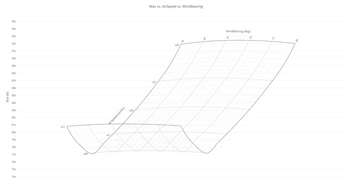
Max vs airspeed vs windbearing carpet plot
This Carpet Plot is easy to read and pretty straightforward. Looking at the wind bearing, fuel consumption slightly rises from 40 degrees and peaks between 56 degrees and 64 degrees. As expected, the lowest amount of fuel consumed is at an airspeed near 448 nautical miles per hour.
Saving your work
Save your work and close out ModelCenter application.
- Bring the Data Explorer window to the front.
- Close the Data Explorer window.
- Click when prompted to close your trade study without saving.
- Close the Carpet Plot Tool.
- Click Save (
 ) to save your ModelCenter workflow.
 - Close the ModelCenter application.
Summary
Your aircraft mission is flying from Joint Base Pearl Harbor-Hickam to Travis Air Force Base. You needed to analyze how wind bearing and airspeed would affect your fuel consumption. You analyzed wind bearing and airspeed using the ModelCenter application using the Parametric Study tool. The preliminary analysis showed that a wind bearing of approximately 60 degrees caused the greatest fuel consumption and 240 degrees the least. Next, you determined that an airspeed of approximately 450 nautical miles per hour consumed the least amount of fuel. Finally, you combined analysis of both wind bearing and airspeed using the Carpet Plot tool to obtain one plot showing the affects of both input variable inputs and how they affect fuel consumption.
On your own
If you have the time, you can create many more steps in the wind bearing and airspeed settings to obtain a much more precise analysis.