STK Pro, STK Premium (Air), STK Premium (Space), or STK Enterprise
You can obtain the necessary licenses for this tutorial by contacting AGI Support at support@agi.com or 1-800-924-7244.
The results of the tutorial may vary depending on the user settings and data enabled (online operations, terrain server, dynamic Earth data, etc.). It is acceptable to have different results.
This tutorial requires version 12.9 of the STK software or newer to complete.
Capabilities covered
This lesson covers the following capabilities of the Ansys Systems Tool Kit® (STK®) digital mission engineering software:
- STK Pro
- Coverage
Problem statement
The oceanic pole of accessibility is a location in the Pacific ocean centered around Point Nemo, the location on Earth farthest from any land. At 2,688 kilometers away from the nearest island, its remoteness and limited shipping traffic makes it a good location for disposing of inactive satellites; as such, this area is known as the satellite graveyard. You want to image the oceanic region around Point Nemo during as part of an upcoming spacecraft de-orbiting procedure. You will use a satellite with an on-board camera to do so. You know the location of Point Nemo, but you need a quick and easy way to model the analysis area and assess the quality of the coverage provided by your satellite. Because your satellite will be collecting surface imagery, you want to assess coverage across the region while the surface of the Earth is at least partially illuminated.
Solution
Use the Coverage capability and the Coverage Tool method to create both a Coverage Definition object and a Figure Of Merit object to compute the coverage over the region and analyze the results. Use Point Nemo as a starting point to create a custom area of interest to model your coverage area in just a few steps, then apply a lighting constraint to the coverage grid to analyze the quality of your coverage.
What you will learn
Upon completion of this tutorial, you will be able to:
- Insert a Coverage Definition object using the Coverage Tool method
- Create a grid area of interest from a starting point object
- Assign a Sensor object as the coverage asset
- Insert a Figure Of Merit object to analyze simple coverage
- Apply lighting conditions to the coverage analysis
- Analyze what percentage of the grid is accessed by the Sensor object
Creating a new scenario
Create a new scenario with a one-day analysis period.
- Launch the STK application (
 ).
). - Click
 Create a Scenario.
 - Enter the following in the STK: New Scenario Wizard:
- Click when you finish.
- Click Save (
 ) when the scenario loads.
 - Verify the scenario name and location shown in the Save As dialog box.
- Click .
| Option | Value |
|---|---|
| Name | Coverage_Tool_Point_Nemo |
| Start | Default |
| Stop | Default |
A folder with the same name as your scenario is created for you.
Save () often!
Turning off streaming terrain
By default, the STK application connects to the Ansys Geospatial Data Cloud to distribute Earth terrain data for analysis and visualization. Turn off
- Right-click on Coverage_Tool_Point_Nemo () in the Object Browser.
- Select Properties (
 ) in the shortcut menu.
 - Select the Basic - Terrain page when the Properties Browser opens.
- Clear the Use terrain server for analysis check box in the Terrain Server panel.
- Click to confirm your change and to close the Properties Browser.
Inserting the imaging satellite
Insert a
- Bring the Insert STK Objects tool (
 ) to the front.
 - Select Satellite (
 ) in the Select An Object To Be Inserted list.
 - Select Orbit Wizard (
 ) in the Select A Method list.
 - Click .
- Open the Type drop-down list when the Orbit Wizard opens.
- Select Sun Synchronous.
- Enter EarthObsSat in the Satellite Name field.
- Click to propagate EarthObsSat () and to close the Orbit Wizard.
Inserting the satellite's imaging camera
Attach a
- Bring the Insert STK Objects tool () to the front.
- Insert a Sensor (
 ) object using the Insert Default () method.
 - Select EarthObsSat () when the Select Object dialog box opens.
- Click to confirm your selection and to close the Select Object dialog box.
- Right-click on Sensor1 () in the Object Browser.
- Select Rename in the shortcut menu.
- Rename Sensor1 () Camera_View.
Inserting Point Nemo
Insert a
- Bring the Insert STK Objects tool () to the front.
- Insert a Place (
 ) object using the Define Properties () method.
 - Select the Basic - Position page when the Properties Browser opens.
- Set the following options in the Position panel:
- Click to confirm your changes and to close the Properties Browser.
- Rename Place1 () Point_Nemo.
| Option | Value |
|---|---|
| Latitude | -48.87 deg |
| Longitude | -123.39 deg |
Viewing the changes
View EarthObsSat in the 3D Graphics window to gain situational awareness with respect to its position relative to Point Nemo.
- Bring the 3D Graphics window to the front.
- Right-click on Point_Nemo () in the Object Browser.
- Select Zoom To in the shortcut menu.
- Zoom out until you can get a good view of the globe.
- Click Start (
 ) on the Animation toolbar to animate your scenario.
 - Click Reset (
 ) when you are finished.
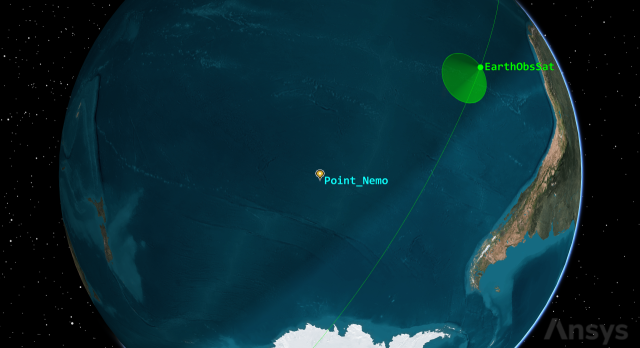
Point Nemo and EarthObsSat
Watch as the field of view of Camera_View passes near and over Point Nemo.
Using the Coverage Tool method
Now that you have your assets modeled in the scenario, use the Coverage Tool, part of the Coverage capability, to analyze the region around Point Nemo. The
Inserting a new Coverage Definition object
Add a new Coverage Definition object using the Coverage Tool method.
- Bring the Insert STK Objects tool () to the front.
- Insert a Coverage Definition (
 ) using the Coverage Tool () method.
Configuring the coverage grid
The statistical data computed during a coverage analysis is based on a set of locations, or points, which span a specified grid area of interest. With the Coverage Tool method, as in other coverage analyses you can select among several types of custom regions to
- Enter Satellite_Graveyard in the Name field when the Coverage Tool opens.
- Leave Area Of Interest selected in the drop-down list in the Regions panel.
- Select Point_Nemo () in the Custom Area Definition list.
- Move (
 ) Point_Nemo () from the Custom Area Definition list to the Selected Regions list.
 - Note that Point_Nemo' s icon changed from to
 when it was added to the Selected Regions list.
 - Leave the type set to Ellipse.
- Enter 2688 km in the Semi-Major Axis field.
- Enter 2688 km in the Semi-Minor Axis field.
- Leave Lat/Lon selected in the Grid Point Granularity panel.
- Enter 2 deg in the Lat/Lon field.
This indicates that the coverage region you are creating is an ellipsoidal shape. If you select Lat/Lon type, the shape will change to  , indicating a box-like pattern.
You are creating a coverage area, which is in the shape of a spherical circle when overlaid on the WGS84 ellipsoid, to cover the entirety of the region to the nearest coastline.
Assigning the coverage asset
Coverage analyses are based on the accessibility of assets (that is, the objects that provide coverage) to the specified geographical area(s). The Coverage Tool method automatically populates the Assets list with all possible objects from the Object Browser that can be assigned to provide coverage. Double-click on Camera_View to assign it to (that is, make it active for) your coverage area.
- Expand (
 ) EarthObsSat () in the Assets list.
 - Double-click on Camera_View () to assign it as your coverage asset.
Assets can only be assigned by double-clicking on them when using the Coverage Tool method. The term (Active) will appear next to an asset when it has been successfully assigned.
Defining the Figure Of Merit object
With the Coverage Tool method, you can specify the method by which the quality of coverage is measured by selecting a
- Confirm that the Type is set Simple Coverage in the FOM Definition panel.
- Click to confirm your changes and to close the Coverage Tool window.
- Rename FigureOfMerit1 (
 ) Simple_Cov.
Note that both a Coverage Definition object and a Figure Of Merit object have been added to the Object Browser.
You can reopen the Coverage Tool by selecting the Coverage Definition object in the Object Browser and then selecting Coverage Tool... in the CoverageDefinition menu. A warning will appear asking you to confirm if you want to allow the Coverage Tool to change the graphics settings.
Viewing the Coverage Definition object in the 3D Graphics window
Take a look at your Coverage Definition object to see your custom area of interest.
- Bring the 3D Graphics window to the front.
- Use your mouse to get a good view of your coverage grid.
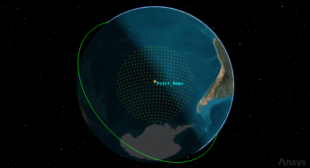
area of interest around Point Nemo
Note that your coverage grid is in a circle around Point_Nemo.
Computing coverage
The ultimate goal of coverage is to analyze accesses to an area using assigned assets and applying necessary limitations upon those accesses. Compute coverage with the
- Select Satellite_Graveyard () in the Object Browser.
- Select the CoverageDefinition menu in the Menu Bar.
- Select Compute Accesses in the CoverageDefinition menu.
The status of the access computations displays in the 2D Graphics window while accesses are being calculated. You can also view the progress of the computations in the
Analyzing the results
The Coverage capability ships with several
Generating a Percent Satisfied report
Generate a
- Right-click on Simple_Cov () in the Object Browser.
- Select Report & Graph Manager... (
 ) in the shortcut menu.
 - Select the Percent Satisfied (
 ) report style, located in the in the Styles Panel list when the Report & Graph Manager opens.
 - Click .
- Note the % Satisfied value at the bottom of the report.
- Minimize the report when finished.
Generating a Grid Stats Over Time graph
A
- Select Grid Stats Over Time (
 ) graph style in the Styles panel list.
 - Click .
- Review the Grid Stats Over Time graph.
- Minimize the Grid Stats over Time graph when finished.
- Close the Report & Graph Manager.
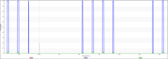
Grid Stats over time
Viewing the Figure Of Merit object
The Figure Of Merit object's
- Open Simple_Cov's () Properties ().
- Select the 2D Graphics - Animation page when the Properties Browser opens.
- Select the Show Animation Graphics check box.
- Open the Show drop-down list in the Accumulation panel.
- Select Up to current time.
- Click to confirm your changes and to close the Properties Browser.
With this method, when animating, grid points that have met the satisfaction criterion based on the dynamic definition of the Figure Of Merit from the start time to the current time are highlighted. Accumulation is only applicable to animation graphics and, therefore, is not available for Figure Of Merit objects without animation behavior.
Visualizing the coverage graphics
View the animated accumulation graphics in the 3D Graphics window.
- Bring the 3D Graphics window to the front.
- Zoom out until you can see the all the grid points.
- Click Start () on the Animation toolbar to animate your scenario.
- Click Reset () when you are finished.
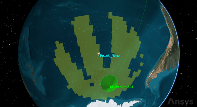
Accumulated Coverage
Watch as Camera_View adds color to the coverage grid along its path as it accesses the grid points.
Accounting for lighting conditions
You can associate
Adding a lighting constraint
- Open Point_Nemo's () Properties ().
- Select the Constraints - Active page when the Properties Browser opens.
- Click Add new constraints (
 ) on the Active Constraints toolbar.
 - Select Lighting in the Constraint Name list when the Select Constraints to Add dialog box opens.
- Click .
- Click to close the Select Constraints to Add dialog box.
- Open the drop-down list in the Lighting panel in the Constraint Properties section.
- Select Penumbra or Direct Sun.
- Click to confirm your changes and to close the Properties Browser.
Applying the lighting constraint
Before the constraints are applied to your coverage grid, you must first specify an object class or a specific object for the points within the grid.
- Open Satellite_Graveyard's () Properties ().
- Select the Basic - Grid page when the Properties Browser opens.
- Click in the Grid Definition panel.
- Open the Reference Constraint Class drop-down list in the Grid Point Access Options panel when the Grid Constraint Options dialog box opens.
- Select Place.
- Select the Use Object Instance check box.
- Select Point_Nemo in the objects list.
- Click to confirm your changes and to close the Grid Constraints Options dialog box.
- Click to confirm your changes and to close Properties Browser.
For all object classes, the Basic properties of the object are applied to the grid points, excluding positional information.
The accesses will automatically be computed. By default, the Automatically Recompute Accesses option is selected in the Coverage Definition object’s
Determining coverage loss
Now that you have added in a constraint, refresh your report and graph to examine the changes.
- Maximize the Percent Satisfied report.
- Click Refresh (F5) (
 ) on the report toolbar.
 - Examine the changes to the report.
- Close the Percent Satisfied report when finished.
- Maximize the Grid Stats Over Time graph.
- Click Refresh (F5) () on the graph toolbar.
- Examine the changes to the graph.
- Close the Grid Stats Over Time graph when finished.

Updated Percent Satisfied Report
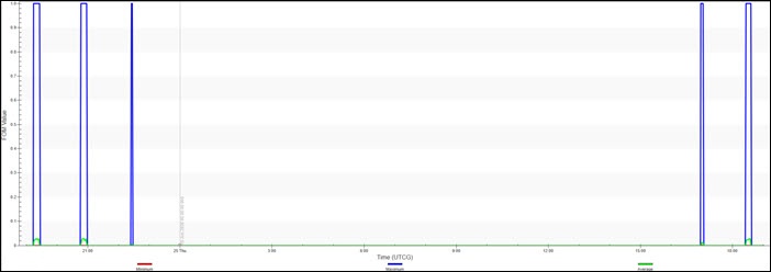
Updated Grid Stats over time Graph
Saving your work
Clean up your workspace and save your scenario.
- Close any open reports, properties and tools.
- Save () your work.
Summary
In this lesson you placed a satellite in a Sun synchronous orbit, then modeled a sensor on it. Then, you created a place object and defined it's position with coordinates of Point Nemo. Once the assets were modeled, you used the Coverage Tool method quickly and easily model a grid area of interest around the point for your Coverage Definition object and insert a Simple Coverage Figure Of Merit object. After examining the results, you incorporated a lighting constraint and refreshed the reports and graphs to see the changes.
On your own
On your own, explore other ways to maximize your coverage. You examined a single day; what if the scenario was longer? What if the satellite had a different orbit? Explore other ways to modify your assets or your Coverage Definition to better understand the mission.