STK Pro, STK Premium (Air), STK Premium (Space), or STK Enterprise
You can obtain the necessary licenses for this tutorial by contacting AGI Support at support@agi.com or 1-800-924-7244.
Required product install: installation of the Navigation Files Plugin, which is included with
The results of the tutorial may vary depending on the user settings and data enabled (online operations, terrain server, dynamic Earth data, etc.). It is acceptable to have different results.
This tutorial requires an internet connection.
Capabilities covered
This lesson covers the following capabilities of the Ansys Systems Tool Kit® (STK®) digital mission engineering software:
- STK Pro
- Coverage
Problem statement
Engineers and operators require a quick way to determine if local terrain is affecting GPS reception for a variety of purposes, such as location, navigation, tracking, mapping, and timing. In this scenario, engineers are performing a training exercise on mountainous terrain in the vicinity of Mount St. Helens. You need to determine the positional uncertainty of the GPS being used to pinpoint their location.
Solution
Use the STK Pro application and the Coverage capability to examine the accuracy of your navigation solution within a specified area based on satellite outages and GPS position uncertainty.
What you will learn
Upon completion of this tutorial, you will understand the following:
- How to determine navigation accuracy
- How to obtain a satellite outage file
- How to use the GPS Satellite Outage tool
- How to use the Navigation Files Plugin
- How to use the Grid Inspector tool
Creating a new scenario
First, you must create a new STK scenario, then build from there.
- Launch the STK application (
 ).
). - Click
 Create a Scenario in the Welcome to STK dialog box.
 - Enter the following in the STK: New Scenario Wizard:
- Click when you finish.
- Click Save (
 ) when the scenario loads.
 - Verify the scenario name and location in the Save As dialog box.
- Click .
| Option | Value |
|---|---|
| Name | NavAccuracy |
| Start | 10 Jan 2020 18:00:00.000 UTCG |
| End | + 1 day |
The STK application automatically creates a folder with the same name as your scenario for you.
Save (![]() ) often during this lesson!
) often during this lesson!
Turning off streaming terrain
By turning off
- Right-click on NavAccuracy () in the Object Browser.
- Select Properties (
 ) in the shortcut menu.
 - Select the Basic - Terrain page when the Properties Browser opens.
- Clear the Use terrain server for analysis check box in the Terrain Server panel.
- Click to confirm your change and to close the Properties Browser.
Adding analytical and visual terrain
An STK terrain inlay (.pdtt) file can be used both for analysis and for visualization in the 3D Graphics window. Use a preinstalled terrain inlay file to your scenario using the
- Bring the 3D Graphics window to the front.
- Click Globe Manager (
 ) on the 3D Graphics window's Globe Manager toolbar.
 - Click Add Terrain/Imagery (
 ) on the Globe Manager Hierarchy toolbar when Globe Manager opens.
 - Select Add Terrain/Imagery... (
 ) in the drop-down menu.
 - Click the Path ellipsis (
 ) when the Globe Manager: Open Terrain and Imagery Data dialog box opens.
 - Browse to the install directory at C:\Program Files\STK_ODTK 13\Data\Resources\stktraining\imagery when the Browse For Folder dialog box opens.
- Click to confirm your selection and to close the Browse For Folder dialog box.
- Select the StHelens_Training.pdtt check box.
- Click .
- Click when prompted to use StHelens_Training.pdtt for analysis.
Viewing the inlaid terrain
View the terrain inlay in the 3D Graphics window.
- Bring the 3D Graphics window to the front.
- Right-click on StHelens_Training.pdtt (
 ) in the Globe Manager hierarchy.
 - Select Zoom To (
 ) in the shortcut menu.
 - Use your mouse to move around and zoom in and out to view the terrain in the 3D Graphics window.
Modeling the training area
Use an Area Target object to outline the training area. An Area Target object models a region on the surface of the central body.
Inserting an Area Target object
Use the Area Target Wizard to add an area target and define its boundaries.
- Go to the Insert STK Objects (
 ) tool.
 - Select Area Target (
 ) in the Select An Object To Be Inserted list.
 - Select Area Target Wizard (
 ) in the Select A Method list.
 - Click .
- Enter ExerciseArea in the Name field when the Area Target Wizard opens.
- Click four times.
- Set the following in the Points panel in the order shown:
- Click to confirm your changes and to close the Area Target Wizard.
| Latitude | Longitude |
|---|---|
| 46.00 deg | -123.00 deg |
| 46.00 deg | -122.00 deg |
| 47.00 deg | -122.00 deg |
| 47.00 deg | -123.00 deg |
Making the area target visible
Earlier in the scenario you turned off steaming terrain. This affects the view of the Area Target object when using a local terrain file. You need to change your Scenario object's properties so you can view the area target on the terrain by turning the display of
- Open NavAccuracy's () Properties ().
- Select the 3D Graphics - Global Attributes page.
- Open the On Terrain drop-down list in the Surface Lines panel.
- Select On.
- Click to confirm your selection and to close the Properties Browser.
Decluttering labels
Objects located on the surface of the terrain could be covered by the terrain, which makes them unreadable. You can fix this by making a change to the 3D Graphics window's properties to enable
- Bring the 3D Graphics window to the front.
- Click Properties () on the 3D Window Defaults toolbar.
- Select the Details page.
- Select the Enable check box in the Label Declutter panel.
- Click to confirm your selection and to close the Properties Browser.
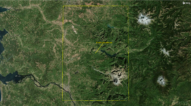
Exercise Area
Loading the GPS constellation
Use the Insert STK Objects tool to
- Return to the Insert STK Objects () tool.
- Insert a Satellite (
 ) object using the Load GPS Constellation (
 ) method.
 - Select gps-23_svn60 () in the Object Browser.
- Click Delete (
 ) on the Object Browser toolbar.
 - Click n the Delete Object dialog box to confirm your deletion.
Once loaded, you will see each individual Satellite (![]() ) object and a Constellation (
) object and a Constellation (![]() ) object containing all of the satellites.
) object containing all of the satellites.
This satellite was decommissioned during the analysis period of the scenario.
Defining a coverage grid
The STK software's Coverage capability allows you to analyze the global or regional coverage provided by one or more assets (facilities, vehicles, sensors, etc.) while considering all accesses. To address area coverage capabilities, the Coverage capability provides you with two STK object classes: Coverage Definition objects and Figure of Merit objects. You will use these objects to analyze navigational accuracy.
Inserting a Coverage Definition object
Before running a coverage analysis, you must first insert a Coverage Definition object. A
- Return to the Insert STK Objects () tool.
- Insert a Coverage Definition (
 ) object using the Insert Default () method.
 - Right-click on CoverageDefinition1 () in the Object Browser.
- Select Rename in the shortcut menu.
- Rename CoverageDefinition1 () PosAccCov.
Choosing the Grid Area of Interest
Coverage analyses are based on the accessibility of assets (objects that provide coverage) and geographical areas. For analysis purposes, you can further refine the geographical areas of interest using regions and points. Points have specific geographical locations, and the STK application uses them in the computation of asset availability. Regions are closed boundaries that contain points. The STK application computes accessibility to a region based on accessibility to the points within that region. The combination of the geographical area, the regions within that area, and the points within each region is called the coverage grid.
- Open PosAccCov's () Properties ().
- Select the Basic - Grid page when the Properties Browser opens.
- Open the Type drop-down list in the Grid Area of Interest panel.
- Select Custom Regions.
- Open the Area Of Interest drop-down list.
- Select Area Targets.
- Select ExerciseArea () in the Area Targets list.
- Move (
 ) ExerciseArea () to the Selected Regions list.
Defining the grid
The statistical data computed during a coverage analysis is based on a set of locations, or points, which span the specified grid area of interest. You can determine the spacing between grid points using the Grid Definition options.
- Open the Lat/Lon drop-down list in the Grid Definition - Point Granularity panel.
- Select Distance.
- Enter 1 mi in the Distance field.
- Open the Altitude above WGS84 drop-down list in the Point Altitude panel.
- Select Altitude above Terrain.
- Leave the default point altitude set to 0 km above the terrain.
- Click to confirm your changes and to close the Properties Browser.
Constraining the coverage grid
Your coverage grid is situated in mountainous terrain. For your analysis to be accurate, each point in your coverage grid needs to take the local terrain into account when computing GPS navigation accuracy. Now that you have defined the grid area, you can specify an object class or a specific object to
You can constrain the grid using an azimuth-elevation (AzEl) mask to model the effects of the terrain. When computing an AzEl Mask from terrain, terrain blockage is only modeled up to the ground distance specified by the maximum range that was considered when generating the mask. The AzEl Mask constraint leverages a provided or computed AzEl Mask to determine visibility; the mask may be computed from terrain information to be representative of terrain-based visibility restrictions.
You can construct terrain-based AzEl masks by extending a number of rays in directions of constant azimuth outwards from the facility, place, or target location. Obstruction information is stored along each ray. During visibility computations, the STK software uses obstruction information from the two rays that bound the current direction of interest to compute an interpolated visibility metric.
Inserting a Place object for a constraint template
Create a Place object to model the AzElMask constraints, which you can then apply to all the points in the coverage grid.
- Return to the Insert STK Objects () tool.
- Insert a Place (
 ) object using the Define Properties () method.
 - Select the Basic - Position page when the Properties Browser opens.
- Enter the following coordinates in the Position panel:
- Click to confirm your changes and to keep the Properties Browser open.
| Option | Value |
|---|---|
| Latitude | 46.5 deg |
| Longitude | -122.5 deg |
These coordinates are close the centroid location of ExerciseArea.
Using an azimuth-elevation mask for analysis
The AzElMask properties enable you to
- Select the Basic - AzElMask page.
- Set the following options:
- Click to confirm your changes and to close the Properties Browser.
- Rename Place1 () ConstraintTemplate.
- Clear the check box for ConstraintTemplate () in the Object Browser.
| Option | Value |
|---|---|
| Use | Terrain Data |
| Max range to consider | 160 km |
| Use Mask for Access Constraint | Selected |
Using Terrain Data automatically creates and stores an AzEl mask file, which is an ASCII text file that is formatted for compatibility with the STK software and ends in an .aem extension, into your scenario folder. Selecting Use Mask for Access Constraint enables the AzEl Mask constraint located on the Constraints - Active page. Using the AzElMask constraint constrains access to a 360-degree field of view around the object being constrained.
You don't need to visualize ConstraintTemplate in the 2D or 3D Graphics windows. The location of the constraints template is unimportant, so long as it is somewhere on the terrain within the area target boundary. You are going to use it to constrain all the points in the coverage grid.
Applying the constraint to the coverage definition
You have a constraint source and you have a defined coverage area. You need to associate the constraint with the points in the grid to which the constraint will be applied.
- Open PosAccCov's () Properties ().
- Select the Basic - Grid page when the Properties Browser opens.
- Click in the Grid Definition panel.
- Open the Reference Constraint Class drop-down list in the Grid Point Access Options panel when the Grid Constraint Options dialog box opens.
- Select Place.
- Select the Use Object Instance check box.
- Select ConstraintTemplate in the list.
- Click to confirm your selection and to close the Grid Constraint Options dialog box.
- Click to confirm your changes and to keep the Properties Browser open.
Using satellite outage files
You've defined and constrained the area within which you'd like to analyze coverage. The next step is to identify your assets. The GPSConstellation Constellation object is the asset with which you want to assess the quality of your coverage. Prior to assigning the GPSConstellation as your asset, however, you need to check for any outages. Satellite outage files (SOFs) provide information about GPS satellite outages. Taking these outages into account is crucial for obtaining an accurate navigation error prediction. Without considering outages, your navigation errors may be smaller than actually observed.
Connecting to the United States Coast Guard Navigation Center website
The U.S. Space Force produces a new SOF each time a new outage is completed, experienced or predicted. You can download the current SOF from U.S. Coast Guard Navigation Center. The SOF provides GPS outage information for historical, current and predicted outages. The SOF provides GPS outage information for historical, current and predicted outages. The historical outages go back to 1998.
- Open your preferred web browser.
- Navigate to the U.S. Coast Guard's Navigation Center's GPS NANUS, Almanacs, OPS Advisories, & SOF page at
- Scroll down to the Satellite Outage File (SOF) section.
- Click the Current SOF - .sof link to download the most recent SOF file, current_sof.sof.
- Close your browser.
Copying the outage file to your scenario folder
Copy the SOF to your scenario folder.
- Navigate to the location of the downloaded current_sof.sof file in Windows File Explorer.
- Copy current_sof.sof.
- Select Documents in the navigation pane.
- Navigate to your scenario folder (for example, C:\Users\<username>\Documents\STK_ODTK 13\TLE_Almanac_Files).
- Paste current_sof.sof in your scenario folder.
- Close Windows File Explorer.
If you chose a non-default folder in which to store your scenarios during the STK application install, you will need to place the current_sof.sof file in your custom location.
Using the GPS Satellite Outage tool
Use the GPS Satellite Outage tool, which is included with the
- Return to the STK application.
- Right-click on GPSConstellation (
 ) in the Object Browser.
 - Select Constellation Plugins in the shortcut menu.
- Select Add GPS Satellite Outages in the Constellation Plugins submenu.
- Increase the size of the GPS Satellite Outage tool window when it opens.
- Click the ellipsis () in the Select GPS Satellite Outage Data panel.
- In the Open dialog box, browse to the location of the SOF file (for example, C:\Users\<username>\Documents\STK_ODTK 13\TLE_Almanac_Files).
- Select current_sof.sof.
- Click .
This will allow you to see the full extent of the tool.
A message noting "Satellite Outage Data Loaded" will appear on the bottom of the Select GPS Satellite Outage Data panel.
You can also access the GPS Satellite Outage tool by clicking Add GPS Satellite Outages ( ) on the Navigation Files Support toolbar (
 ). You can enable the toolbar by selecting Toolbars in the View menu, then selecting Navigation Files Support in the Toolbars submenu.
Applying the outages to the GPS Constellation
With your SOF file loaded, apply the outage to the GPS constellation.
- Ensure GPSConstellation is selecting in the Apply to Which GPS Constellation? list.
- Click .
- Read the message that satellite outage data has been updated in the Update Complete dialog box.
- Click to close the message.
- Review the outage information in the Outage Results Applied panel.
- Click to close the GPS Satellite Outage tool.
The outages for your scenario are determined by your scenario's time frame. Once applied, the text box at the bottom of the tool will list any outages for your scenario. If an outage is found, the tool will list the interval of the outage. The identification of the GPS satellite is based on the PRN assigned to it, which is matched to the space vehicle identifier (SVID) value in the SOF.
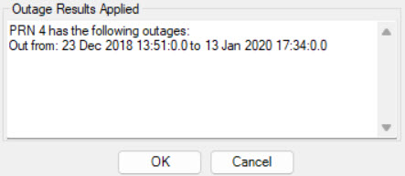
GPS Outage found
If an outage is reported, the STK application will remove the satellite from your analysis by creating a temporal constraint. You can open the satellite's properties and go to the Constraints - Active page. An Intervals constraint will already exist in the Active Constraints list. In the Intervals constraints Constraint Properties list, the outage interval from the SOF will automatically be loaded.
Assigning coverage assets
Now that you've added the SOF to the GPS Constellation use it as the asset providing coverage in your coverage definition. The Coverage Definition Assets properties enable you to
- Return to PosAccCov's () Properties ().
- Select the Basic - Assets page.
- Select GPSConstellation () in the Assets list.
- Click .
- Click to confirm your selection and to keep the Properties Browser open.
Turning off the automatic re-computation of accesses
The STK application automatically recomputes accesses every time you update an object on which the coverage definition depends (such as an asset). If you want control as to when STK computes coverage, you need to turn this off The Coverage Definition's object's
- Select the Basic - Advanced page.
- Clear the Automatically Recompute Accesses check box in the Access panel.
- Click to confirm your change and to close the Properties Browser.
Using the Compute Accesses tool
The ultimate goal of coverage is to analyze accesses to an area by using assigned assets and applying necessary limitations upon those accesses. Compute coverage with the Compute Accesses tool.
- Select PosAccCov () in the Object Browser.
- Select the CoverageDefinition menu in the Menu Bar.
- Select Compute Accesses in Parallel in the CoverageDefinition menu.
Since you have a large amount of grid points and you're using a terrain constraint,
Measuring the accuracy of a navigation solution
You can evaluate navigation accuracy by attaching a Figure of Merit object to the coverage definition of interest. A Navigation Accuracy Figure of Merit considers the effect of the number of measurements (of those satellites visible at each moment in time), the geometry of the transmitters and the uncertainty in the one-way range measurements in the computation of the uncertainty in the navigation solution. The uncertainty in the one-way range measurements may be specified as a constant value or as a function of the elevation angle on a transmitter basis.
Inserting a Figure of Merit object
Attach a
- Return to the Insert STK Objects () tool.
- Insert a Figure Of Merit (
 ) object using the Insert Default () method.
 - Select PosAccCov () when the Select Object dialog box opens.
- Click to confirm your selection and to close the Select Object dialog box.
- Rename FigureOfMerit1 () NavAcc.
Measuring the accuracy of a navigation solution
To evaluate coverage quality, you will first need to set basic parameters that determine the way in which quality is computed. This involves choosing the method for evaluating the quality of coverage provided, setting measurement options and identifying the criterion needed to achieve satisfactory coverage.
- Open NavAcc's () Properties ().
- Select the Basic - Definition page when the Properties Browser opens.
- Open the Type drop-down list in the Definition panel.
- Select Navigation Accuracy.
- Set the following Navigation Accuracy options:
- Click to confirm your changes and to keep the Properties Browser open.
| Option | Value |
|---|---|
| Compute | Maximum |
| Method | PACC |
| Type | Over Determined |
| Time Step | 60 sec |
Viewing navigation uncertainties
Uncertainty exists in any navigation solution. You cannot eliminate uncertainty; you can, however, account for it.
- Click in the Definition panel.
- View the Asset Range Uncertainty and Receiver Range Uncertainty for your GPS satellites when the Figure of Merit NA Uncertainties Model dialog box opens.
- Click to close the Figure of Merit NA Uncertainties Model dialog box.
- Click to close the Properties Browser.
The STK application defaults the Asset and Receiver Range Uncertainties to one meter and zero meters for each satellite.
Checking asset range uncertainty
The GPS constellation experiences errors in its ephemeris (position in space) and clock data that translate into positioning errors in GPS receivers. Knowing these uncertainties helps provide a better prediction of your GPS receiver's accuracy. Navigation uncertainties are directly related to your GPS receiver's navigation accuracy.
Opening the Navigation Files Plugin
Use the
- Right-click on NavAcc () in the Object Browser.
- Select FigureOfMerit Plugins in the shortcut menu.
- Select Add Navigation Uncertainties in the FigureOfMerit submenu.
You can also access the Navigation Files Plugin by clicking Add Navigation Uncertainties ( ) on the Navigation Files Support toolbar ().
Using the Navigation Files Plugin
Using Prediction Support Files (PSFs), you can model your navigation accuracy with higher fidelity. PSFs provide statistical error data for both GPS ephemeris and satellite clock errors. There is a Prediction Support File (PSF) containing GPS satellite errors located in the STK application install that you can use for this scenario.
- Increase the size of the Add Navigation Uncertainties window when it opens.
- Click the ellipsis () in the GPS Satellites panel.
- Browse to C:\Program Files\AGI\STK_ODTK 13\Data\Resources\stktraining\samples.
- Select uncertainties.psf.
- Click .
- Ensure the PosAccCov/NavAcc FOM check box is selected in the Apply to Which Navigation FOMs? panel.
- Click .
- Click to confirm and to close the Asset Anomalies dialog box.
- Click to close Update Complete dialog box.
- Click to close the Add Navigation Uncertainties window.
Note that a message reading "Uncertainty Data Loaded" has appeared in the GPS Satellites panel.
An Asset Anomalies message appears, noting that "Assets with these PRNS are not in the PSF File and have not been updated: 4." The message refers to gps-04_svn74. This is the satellite with the reported outage.
A message in the Update Complete dialog box reading "Satellite and receiver uncertainties have been updated." will be displayed.
Viewing the updated uncertainties
The STK application has the ability to use this data on the Navigation Accuracy Figure of Merit properties page. View the updated uncertainties that you applied to your figure of merit.
- Open NavAcc's () Properties ().
- Select the Basic - Definition page when the Properties Browser opens.
- Click in the Definition Panel.
- Look in the Asset Range Uncertainty panel in the Figure of Merit NA Uncertainties Model dialog box.
- Look in the Receiver Range Uncertainty panel.
- Click to close the Figure of Merit NA Uncertainties Model dialog box.
- Click to close the Properties Browser without making any changes.
You will notice the constant value for each satellite has been updated with values from the PSF file.
The values have likewise been adjusted.
Assessing position accuracy with a custom report
You can assess the position accuracy by
Duplicating the installed report style
A
- Right-click on NavAcc () in the Object Browser.
- Select Report & Graph Manager... (
 ) in the shortcut menu.
 - Right-click on the Grid Stats Over Time (
 ) report in the Installed Styles (
 ) folder of the Styles panel when the Report & Graph Manager opens.
 - Select Duplicate (
 ) in the shortcut menu.
Setting the minimum summary option
Summary options allow you to refine a report to make it easier to find minimum and maximum values for selected data provider elements. Start by setting the minimum summary option.
- Select the Content page when the Properties Browser opens.
- In the Report Contents list, select Overall Value by Time - Minimum.
- Click .
- In the Summary Options - Statistics panel, select the Min check box when the Options dialog box opens.
- Click to confirm your change and to close the Options dialog box.
This will display the Minimum value of the Minimum column of FOM data.
Setting the maximum summary option
Now, set up the maximum summary option.
- Select Overall Value by Time - Maximum.
- Click .
- In the Summary Options-Statistics panel, select the Max check box when the Options dialog box opens.
- Click to confirm your change and to close the Options dialog box.
- Click to confirm your selections and to close the Properties Browser.
This will display the Maximum value of the Maximum column of FOM data.
Generating the custom report
Rename and generate your custom report.
- Right-click on Grid Stats Over Time (
 ) in the My Styles () folder.
 - Select Rename in the shortcut menu.
- Rename Grid Stats Over Time () My Grid Stats Over Time.
- Click .
- Scroll through the report.
- Look at the different sections.
- Scroll to the bottom of the report.
- Close the report and the Report & Graph Manager.
Be patient. The report could take a couple of minutes to generate.
First is the Coverage Properties section, which simply shows values from the Coverage Definition object. Next is the FOM properties section, which shows the asset range uncertainties for each GPS satellite and the minimum, maximum, and average uncertainties in meters over time.
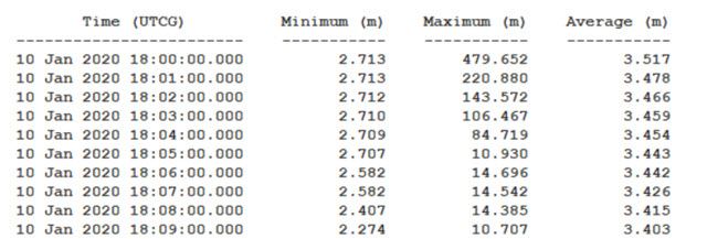
Grid Stats Over Time
You will see the min minimum, max maximum, and average uncertainties in meters.
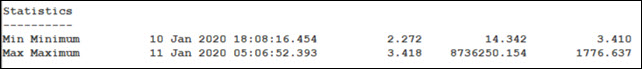
Global Statistics
The min and max values can be useful when deciding on contour levels for visualizing data.
Visualizing the navigation uncertainties
You can set the
Specifying contour graphics
Specify how levels of coverage quality display in both the 2D and 3D Graphics windows using contour graphics. Contour levels represent the gradations in coverage quality and can be displayed for both static and animation values of the figure of merit. Since these values change over the 24-hour analysis period, you'll focus on
- Open NavAcc's () Properties ().
- Select the 2D Graphics - Animation page when the Properties Browser opens.
- Enter 30 in the Filled Area - % Translucency field in the Show Points As panel.
- Select the Show Contours option in the Display Metric panel.
- Click in the Level Attributes panel.
- Enter the following options in the Level Adding panel:
- Click .
- Set the following in the Level Attributes panel:
- Select the Natural Neighbor option in Contour Interpolation (points must be filled) panel.
- Click to confirm your changes and to keep the Properties Browser open.
| Option | Value |
|---|---|
| Level Adding - Start | 0 m |
| Level Adding - Stop | 10 m |
| Level Adding - Step | 1 m |
For the purposes of this exercise, any range uncertainty greater than 10 meters will be considered unacceptable.
| Option | Value |
|---|---|
| Color Method | Color Ramp |
| Start Color | Blue |
| End Color | Red |
Displaying the Legend window
Insert a legend display in the 2D and 3D Graphics windows.
- Click in the Level Attributes panel.
- Click when the Animation Legend for NavAcc window opens.
- Select the Show at Pixel Location check box in the 2D Graphics Window panel when the Figure of Merit Legend Layout dialog box opens.
- Select the Show at Pixel Location check box in the 3D Graphics Window panel.
- Enter Meters in the Title field in the Text Options panel.
- Enter 0 in the Number Of Decimal Digits field.
- Enter 50 in the Color Square Width (pixels) field in the Range Color Options panel.
- Click to confirm your changes and to close the Figure of Merit Legend Layout dialog box.
- Close the Animation Legend for NavAcc window.
- Click to close the Properties Browser.
Viewing the navigation uncertainties in the 3D Graphics window
During the 24 hour period, you can visualize, based on color contours, how your range uncertainties are changing. Any time an area turns red, you are at or above your cutoff uncertainty of 10 meters.
- Bring the 3D Graphics window to the front.
- Click Start (
 ) in the Animation toolbar to animate your scenario.
 - Click Reset (
 ) when finished.
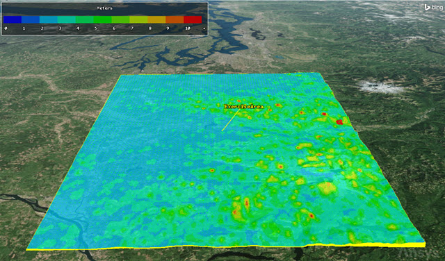
Range Uncertainties
You can see the range uncertainties change over time.
Inspecting regions and points with the Grid Inspector
If you know exactly where the test team is located, you can use the Grid Inspector tool, which enables you to focus more closely on a region or point within a coverage grid, to learn more about a specific location, furthering your analysis efforts.
Opening the Grid Inspector tool
Open the Grid Inspector with the NavAcc Figure of Merit object.
- Bring the 2D Graphics window to the front.
- Zoom In (
 ) to the exercise area.
 - Clear the NavAcc () check box in the Object Browser.
- Right-click on NavAcc () in the Object Browser.
- Select FigureOfMerit in the shortcut menu.
- Select Grid Inspector... (
 ) in the FigureOfMerit submenu.
This enables you to see the grid points more easily inside the area target.
The Grid Inspector tool will open.

Grid Inspector TOol
Using the Grid Inspector
For a Figure Of Merit object , the Grid Inspector provides detailed quality-related information.
- Click a grid point in the 2D Graphics window.
- Look at the information in the Messages panel.
Reviewing the Point Figure of Merit graph
There are several
- Click in the Graphs panel.
- Place your cursor at the top of any spikes in your graph.
- Read the date and time that the navigation accuracy spikes.
- Close the Point Figure of Merit graph when you are finished.
- If desired, try different points.
- Click to close the Grid Inspector tool when finished.
A
Saving your work
Clean up your workspace and save your work.
- Close any open reports, properties and tools.
- Save () your work.
Summary
You began by adding a local terrain inlay file (*.pdtt) to be used both analytically and visually. Next, you defined the area of interest (ExerciseArea) by inserting an Area Target object. After inserting the GPS satellite constellation, you created a Coverage Definition object that focused on ExerciseArea. Prior to assigning coverage assets, you download a satellite outage file and used the GPS Satellite Outage tool to create a temporal constraint on one of the GPS satellites. After assigning the GPS constellation as a coverage asset and computing coverage, you inserted a Figure of Merit object and set it up to report on Navigation Accuracy using the Position Accuracy figure of merit type. To add realism to the analysis, you downloaded the actual range uncertainty file for the analysis time period and used the Navigation Files plugin to quickly update the asset range and receiver range uncertainties. Next you created a custom report that added minimum and maximum global statistics to an existing report style. After adding contour colors specific to positional accuracy to both the 2D and 3D Graphics windows, you explored the function of the Grid Inspector tool.