STK Pro, STK Premium (Air), STK Premium (Space), or STK Enterprise
You can obtain the necessary licenses for this tutorial by contacting AGI Support at support@agi.com or 1-800-924-7244.
The results of the tutorial may vary depending on the user settings and data enabled (online operations, terrain server, dynamic Earth data, etc.). It is acceptable to have different results.
This lesson requires STK 12.8 or newer to complete in its entirety. If you have an earlier version of STK, you can view a legacy version of this lesson.
Capabilities covered
This lesson covers the following STK Capabilities:
- STK Pro
- Communications
Problem statement
Engineers and operators need to analyze laser communication link budgets using propagation losses at optical and IF frequency ranges. Weather conditions (such as humidity, clouds, fog, or dust) affect these propagation losses. The main advantage of using laser communications rather than using radio waves is increased bandwidth. Increased bandwidth enables the transfer of more data in less time. Laser communications can connect satellite to satellite, ground application to satellite, or satellite to ground application.
In this lesson, you will design a laser communications system. You will evaluate a multi-hop satellite to satellite and satellite to ground laser communications link.
Solution
You will use STK Pro and STK's Communications capabilities to model and analyze a link budget between a Low Earth Orbiting (LEO) satellite, a Geosynchronous satellite (Geo), and a ground site. You will use both the Beer-Bouguer-Lambert Law and the MODTRAN-derived Lookup Table Laser Atmospheric Absorption Loss Models to design the laser communications link.
What you will learn
Upon completion of this lesson, you will understand the following:
- Laser receiver and transmitter models
- Laser environment properties
- Multi-hop communications
Video guidance
Watch the following video. Then follow the steps below, which incorporate the systems and missions you work on (sample inputs provided).
Creating a new scenario
Create a new scenario.
- Launch STK (
 ).
). - Click
 Create a Scenario in the Welcome to STK dialog box.
 - Enter the following in the STK: New Scenario Wizard:
- Click when you finish.
- Click Save (
 ) when the scenario loads. STK creates a folder with the same name as your Scenario () object for you.
 - Verify the scenario name and location in the Save As window.
- Click .
| Option | Value |
|---|---|
| Name: | STK_Laser_Comms |
| Location: | Default |
| Start: | 1 Mar 2022 20:00:00.000 UTCG |
| Stop: | 2 Mar 2022 20:00:00.000 UTCG |
Save (![]() ) often during this lesson!
) often during this lesson!
Disabling Terrain Server
Terrain will not be used in your analysis, so you can turn off the Terrain Server:
- Right- click on STK_Laser_Comms () in the Object Browser.
- Select Properties (
 ).
). - Select the Basic - Terrain page when the Properties Browser opens.
- Clear the Use terrain server for analysis check box.
- Click to accept your change and to close the Properties Browser.
Inserting a LEO satellite
The International Space Station (ISS) will transmit laser communications to a Geo satellite. You will insert the ISS from the online Satellite Database.
- Select Satellite (
 ) in the Insert STK Objects tool.
 - Select the From Standard Object Database (
 ) method.
 - Click .
- Enter 25544 in the Name or ID: field within the Search Standard Object Data dialog box.
- Click .
- Select ISS (ZARYA) in the Results: list.
- Click .
- Click to close the Search Standard Object Data dialog box after ISS_ZARYA_25544 () propagates.
Inserting a Geo satellite
The Geo satellite will relay laser communications from the ISS to a ground site.
- Insert a Satellite () object using the Orbit Wizard (
 ) method.
 - Set the following in the Orbit Wizard:
- Click to propagate Geo_Sat () and to close the Orbit Wizard.
| Option | Value |
|---|---|
| Type: | Geosynchronous |
| Satellite Name: | Geo_Sat |
| Subsatellite Point: | -130 deg |
Inserting a ground site
You have selected a ground site location that is located in desert terrain and has a clear atmosphere throughout most of the year.
- Insert a Place (
 ) object using the Define Properties () method.
 - Select the Basic - Position page when the Properties Browser opens.
- Set the following in the Position panel:
- Click to accept your changes and to close the Properties Browser.
- Right-click on Place1 () in the Object Browser.
- Select Rename in the shortcut menu.
- Rename Place1 () to Ground_Site.
| Option | Value |
|---|---|
| Latitude: | 34.382 deg |
| Longitude: | -117.682 deg |
| Height Above Ground: | 10 ft |
Creating an ISS transmitter antenna gimbal system
Laser communications require high antenna gain. However, maintaining contact with extremely narrow beams is difficult, especially if transmitters and receivers change their relative positions. Laser communications require a two-dimensional gimbal to achieve precise alignment, tracking, and pointing. In STK, you use a Sensor (![]() ) object to model this.
) object to model this.
- Insert a Sensor (
 ) object using the Insert Default (
 ) method.
 - Select ISS_ZARYA_25544 () in the Select Object dialog box.
- Click to close the Select Object dialog box.
- Rename the Sensor1 () to ISS_Tx_Antenna_Gimbal.
Modifying the sensor's field of view
Use a Simple Conic sensor pattern. When using the Sensor (![]() ) object to point the antenna at a target, you can use the sensor's field of view for situational awareness. It's up to you to define that view.
) object to point the antenna at a target, you can use the sensor's field of view for situational awareness. It's up to you to define that view.
- Open ISS_Tx_Antenna_Gimbal's () properties ().
- Select the Basic - Definition page when the Properties Browser opens. The default Sensor Type: is set to Simple Conic.
- Enter 1 deg in the Cone Half Angle: field in the Simple Conic panel.
- Click to accept your change and to keep the Properties Browser open.
Targeting the Geo satellite
The Sensor's Pointing page enables you to set parameters to determine how a sensor is aimed. The Targeted pointing type causes the sensor to point to other objects in the scenario. In this case, you will point to (or target) GEO_Sat (![]() ).
).
- Select the Basic - Pointing page.
- Open the Pointing Type: shortcut menu.
- Select Targeted.
- Open the Track Mode: shortcut menu in the Targeted panel.
- Select Transmit.
- Select Geo_Sat (
 ) in the Available Targets list.
 - Move (
 ) Geo_Sat () to the Assigned Targets list.
 - Click to accept your changes and to close the Properties Browser.
Adding a laser transmitter to the ISS
You will set up the International Space Station's laser transmitter.
- Insert a Transmitter (
 ) object using the Insert Default () method.
 - Select ISS_Tx_Antenna_Gimbal () in the Select Object dialog box.
- Click to close the Select Object dialog box.
- Rename Transmitter1 () to Uplink_Tx.
Laser transmitter model
The Laser Transmitter model models the transmit terminal of a laser communications link. In combination with the Laser Receiver model, it facilitates communications laser link budget analysis.
- Open Uplink_Tx's () properties ().
- Select the Basic - Definition page when the Properties Browser opens.
- Click the Transmitter Model Component Selector (
 ).
). - Select Laser Transmitter Model (
 ) in the Select Component dialog box.
 - Click to close the Select Component dialog box.
- Click to accept your change and to keep the Properties Browser open.
Using Model Specs
The Model Specs tab allows you to set the transmitter's frequency, power and data rate.
- Select the Model Specs tab.
- Set the following:
- Click to accept your changes and to keep the Properties Browser open.
| Option | Value |
|---|---|
| Frequency: | 101 THz |
| Power: | 20 dBW |
| Data Rate: | 1.2 Gb/sec |
Transmitter antenna
The Gaussian Optical Antenna Model uses an analytical model of a Gaussian beam. The model is like a parabolic antenna within about -6 dB relative to the boresight. This antenna is specific to a laser transmitter or receiver.
- Select the Antenna tab. The default antenna model is Gaussian Optical.
- Set the following:
- Click to accept your changes and to close the Properties Browser.
| Option | Value |
|---|---|
| Design Frequency: | 101 THz |
| Gain: | 85 dB |
Copying scenario objects
To save time, you can reuse scenario objects in STK. Keep in mind that any objects which you reuse will also copy any attached objects. Copy the ISS_Tx_Antenna_Gimbal (![]() ) and paste it onto the Geo_Sat (
) and paste it onto the Geo_Sat (![]() ).
).
- Right-click on ISS_Tx_Antenna_Gimbal () in the Object Browser.
- Select Copy (
 ) in the shortcut menu.
 - Right-click Geo_Sat () in the Object Browser.
- Select Paste (
 ) in the shortcut menu.
 - Right-click Uplink_Tx1 () in the Object Browser.
- Select Delete (
 ) in the shortcut menu.
 - Click in the Delete Object dialog box.
- Rename ISS_Tx_Antenna_Gimbal1 () to Geo_Rx_Antenna_Gimbal.
Pointing to the ISS
You need to point Geo_Rx_Antenna_Gimbal (![]() ) at ISS_ZARYA_25544 (
) at ISS_ZARYA_25544 (![]() ) to establish a connection.
) to establish a connection.
- Open Geo_Rx_Antenna_Gimbal's () properties ().
- Select the Basic - Pointing page when the Properties Browser opens.
- Open the Track Mode: shortcut menu in the Targeted panel.
- Select Receive.
- Select ISS_ZARYA_25544 () in the Available Targets list.
- Move () ISS_ZARYA_25544 () to the Assigned Targets list.
- Click to accept your changes and to close the Properties Browser.
Adding a laser receiver to Geo_Sat
You need to attach a Receiver (![]() ) object to GEO_Rx_Antenna_Gimbal (
) object to GEO_Rx_Antenna_Gimbal (![]() ).
).
- Insert a Receiver (
 ) object using the Insert Default () method.
 - Select GEO_Rx_Antenna_Gimbal () in the Select Object dialog box.
- Click to close the Select Object dialog box.
- Rename Receiver1 () to Uplink_Rx.
Laser Receiver model
The Laser Receiver model enables you to model free space laser communications in the near infrared, visual, and ultraviolet bands.
- Open Uplink_Rx's () properties ().
- Select the Basic - Definition page when the Properties Browser opens.
- Click the Receiver Model Component Selector ().
- Select Laser Receiver Model () in the Select Component dialog box.
- Click to close the Select Component dialog box.
Using Model Specs
The Model Specs tab allows you to set the Frequency, Optical Detector Specifications and Link Margin.
- Select the Model Specs tab.
- Look at the default settings on this page.
- Click to accept your change and to keep the Properties Browser open.
The Auto Track option allows a receiver to track and lock onto the transmitter's carrier frequency with which it is currently linking, including any Doppler shift.
APD Photodetector computes the signal-to-noise ratio. An APD photodetector differs from a PIN photodetector by providing internal signal gain.
Choosing an antenna model
Use the Gaussian Optical Antenna Model.
- Select the Antenna tab. The default antenna model is the Gaussian Optical antenna model.
- Set the following:
- Click to accept your changes and to close the Properties Browser.
| Option | Value |
|---|---|
| Design Frequency: | 101 THz |
| Gain: | 85 dB |
You have established a two-way connection between the satellites and can analyze a link budget.
Creating a simple Link Budget
You can create a Simple Link Budget report with the Access tool. The Link Budget Report is a specialized Access Report for basic link budget analysis and is available using the Link Budget button in the Reports panel of the Access window. Throughout the rest of the lesson, you will make Link Budget reports to show Bit Error Rates (BER) and you will refresh the reports as you modify the scenario.
- Right-click on Uplink_Rx () in the Object Browser.
- Select Access... (
 ) in the shortcut menu.
 - Expand (
 ) ISS_ZARYA_25544 () in the Associated Objects list when the Access tool opens.
 - Expand () ISS_Tx_Antenna_Gimbal ().
- Select Uplink_Tx ().
- Click
 .
.
Generating a Link Budget report
- Click in the Reports panel.
- Scroll to the right of the report.
- Locate the BER (Bit Error Rate) column.
- Scroll down through the report.
- When finished, close the report and the Access Tool.
You require a BER of 1.000000e-08 or lower. The satellite-to-satellite optical transmission occurs in outer space. At this point, your BER values, overall, are good.
Relaying the satellite-to-satellite transmission to the ground site
Your link budget in outer space is good. Re-transmitting the signal from Geo_Sat (![]() ) to Ground_Site (
) to Ground_Site (![]() ) adds a new dimension: atmosphere.
) adds a new dimension: atmosphere.
- Right-click on ISS_Tx_Antenna_Gimbal () in the Object Browser.
- Select Copy () in the shortcut menu.
- Right-click Geo_Sat () in the Object Browser.
- Select Paste () in the shortcut menu.
- Rename ISS_Tx_Antenna_Gimbal1 () to Geo_Tx_Antenna_Gimbal.
Targeting the ground site
- Open Geo_Tx_Antenna_Gimbal's () properties ().
- Select the Basic - Pointing page when the Properties Browser opens.
- Select Ground_Site () in the Available Targets list.
- Move () Ground_Site () to the Assigned Targets list.
- Click to accept your change and to close the Properties Browser.
- Rename Uplink_Tx1 () to Downlink_Tx.
Using Model Specs
You need to update Downlink_Tx's (![]() ) Model Specs.
) Model Specs.
- Open Downlink_Tx's () properties ().
- Select the Model Specs tab.
- Enter 100 THz in the Frequency: field.
- Click to accept your change and to keep the Properties Browser open.
Antenna specs
You need to update Downlink_Tx's (![]() ) antenna specs.
) antenna specs.
- Select the Antenna tab.
- Select the Model Specs tab.
- Enter 100 THz in the Design Frequency: field.
- Click to accept your change and to close the Properties Browser.
Ground site receiver antenna gimbal system
Next, you need to set up Ground_Site's (![]() ) antenna gimbal system. Ground_Site (
) antenna gimbal system. Ground_Site (![]() ) will target Geo_Sat (
) will target Geo_Sat (![]() ).
).
- Right-click Geo_Rx_Antenna_Gimbal () in the Object Browser.
- Select Copy () in the shortcut menu.
- Right-click Ground_Site (
 ) in the Object Browser.
 - Select Paste () in the shortcut menu.
- Rename Geo_Rx_Antenna_Gimbal1 () to GS_Rx_Antenna_Gimbal.
Targeting the GEO satellite
- Open GS_Rx_Antenna_Gimbal's () properties ().
- Select the Basic - Pointing page when the Properties Browser opens.
- Select ISS_ZARYA_25544 () in the Assigned Targets list.
- Remove (
 ) ISS_ZARYA_25544 () from the Assigned Targets list.
 - Select Geo_Sat () in the Available Targets list.
- Move () Geo_Sat () to the Assigned Targets list.
- Click to accept your changes and to close the Properties Browser.
- Rename Uplink_Rx1 () to Downlink_Rx.
Updating antenna specs
Update Downlink_Rx's (![]() ) antenna specs.
) antenna specs.
- Open Downlink_Rx's () properties ().
- Select the Basic - Definition page when the Properties Browser opens.
- Select the Antenna tab.
- Select the Model Specs tab.
- Enter 100 THz in the Design Frequency: field.
- Click to accept your changes and to keep the Properties Browser open.
Viewing the entire link
You can visualize the entire link in the 3D Graphics window.
- Bring the 3D Graphics window to the front.
- Click Start (
 ) on the Animation Toolbar to animate your scenario.
 - Click Pause (
 ) to pause the scenario when you can see the uplink and the downlink.
 - Click Reset (
 ) when finished.
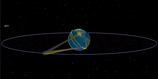
Uplink and Downlink View
Laser environment Beer-Bouguer-Lambert Law model
You will test your satellite to ground link budget using two laser environment models: The Beer-Bouguer-Lambert Law model and the MODTRAN-derived Lookup Table. Start with the Beer-Bouguer-Lambert Law model.
The Beer-Bouguer-Lambert Law defines the attenuation of an optical signal traveling through an optically homogeneous medium, based on propagation distance and an extinction coefficient specific to medium and signal. STK's implementation allows you to divide the atmosphere into concentric homogeneous spheres, or layers, each having different optical properties. The propagation loss for each layer is then computed using the Beer-Bouguer-Lambert Law.
- Return to Downlink_Rx's () properties ().
- Select the Laser - Environment page.
- Select the Atmospheric Loss tab.
- Select the Enable check box.
- Ensure Beer-Bouguer-Lambert Law is the Laser Atmospheric Absorption Loss Model.
- Click Apply to accept your change and to keep the Properties Browser open.
Using atmospheric layers in STK
You will create three atmospheric layers, studying the effects of each one on your link budget. A lower atmospheric layer has a higher extinction coefficient. The extinction coefficient is how quickly the signal will attenuate through a homogenous medium. Extinction can come from molecular absorption, scattering, and aerosol scattering.
Since the atmosphere has characteristic profiles that vary with altitude (such as temperature, pressure, humidity, and various aerosol content), you can model these vertical profile characteristics with multiple concentric spheres. You can make each concentric sphere have a different extinction coefficient based on the condition of that layer of the atmosphere being modeled.
The number of layers depends on the level of fidelity you want to model. You could just simply model the entire atmosphere with some averaged extinction rate based on a generalized condition, or you can model many layers each with a different extinction. If you don't know the extinction coefficient, you may know the transmittance and the range. Given these two, you can calculate the extinction coefficient. For instance, if you operate within one layer of the atmosphere and you know the transmittance is 93 percent for a path of 5 kilometers, then the extinction coefficient would be 1.45e-5.
For now, you can keep things simple to learn how this feature works.
Adding atmospheric layer 1
You can set up the first atmospheric layer.
- Notice by default the top of layer number 1 is at an altitude of 100 km.
- Double-click in the ExtinctionCoefficient cell of layer number 1.
- Set the value to 1e-07 m^-1.
- Click to accept your changes and to keep the Properties Browser open.
Creating a simple Link Budget
As you continue to make changes to the atmospheric conditions of the scenario, you can refresh a Link Budget report to see how those atmospheric changes affected the scenario. You will generate a Link Budget Report to look at the BER between Ground_Site's (![]() ) receiver and the Geo_Sat's (
) receiver and the Geo_Sat's (![]() ) transmitter.
) transmitter.
- Right-click on Downlink_Rx () in the Object Browser.
- Select Access... () in the shortcut menu.
- Expand () Geo_Sat () in the Associated Objects list when the Access tool opens.
- Expand () Geo_Tx_Antenna_Gimbal ().
- Select Downlink_Tx ().
- Click .
Generating a link budget report
- Click in the Reports panel.
- Scroll to the right of the report.
- Locate the BER column.
- Scroll down through the report.
- Notice that the BER rates are below 1.000000e-08.
- Keep the Link Budget report open.
Adding atmospheric layer 2
Here, you can set up the second atmospheric layer.
- Return to Downlink_Rx's () properties ().
- Click .
- Notice that layer 1 was renamed to layer 2 and the top of the new layer 1 is set to an altitude of 50 km.
- Double-click in the ExtinctionCoefficient cell for the new layer 1.
- Set the value to 1e-06 m^-1.
- Click to accept your change and to keep the Properties Browser open.
Refreshing the Link Budget report
By refreshing the report, you can see how atmospheric layer 2 affected the scenario. You will repeat this process throughout the lesson so you can better analyze the scenario.
- Return to the Link Budget report.
- Click Refresh (F5) (
 ) in the report's toolbar.
 - Scroll through your BER column.
- Keep the Link Budget report open.
Adding a second layer had some impact to your link budget but the BER values are still good.
Adding atmospheric layer 3
Set up a third atmospheric layer.
- Return to Downlink_Rx's () properties ().
- Select the last layer in the list.
- Click .
- Notice layer 1 was renamed to layer 2, layer 2 to layer 3, and the new layer is layer 1.
- Notice STK automatically changed the second layer's altitude to 66.6667 km.
- Notice that the top of the new layer 1 is at an altitude of 33.3333 km.
- Double-click in the ExtinctionCoefficient cell for the new layer 1.
- Set the value to 1e-05 m^-1.
- Click to accept your change and to keep the Properties Browser open.
Refreshing the Link Budget report
- Return to the Link Budget report.
- Click Refresh (F5) () in the report's toolbar.
- Scroll through your BER column.
- Keep the Link Budget report open.
The lower layer had a significant impact on the link budget BERs which are now above the cutoff of 1.000000e-08.
Increasing the antenna gain
Increase the receiver's antenna gain to 86 dB.
- Return to Downlink_Rx's () properties ().
- Select the Basic - Definition page.
- Select the Antenna tab.
- Enter 86 dB in the Gain: field.
- Click to accept your change and to keep the Properties Browser open.
Refreshing the Link Budget report
Analyze the increased gain's effect on your BERs.
- Return to the Link Budget report.
- Click Refresh (F5) () in the report's toolbar.
- Scroll through your BER column.
- Keep the Link Budget report open.
The 1 dB gain increase lowered the BERs to an acceptable level.
Resetting the receiver antenna's gain
Reset the receiver's gain to 85 dB.
- Return to Downlink_Rx's () properties ().
- Select the Basic - Definition page.
- Select the Antenna tab.
- Enter 85 dB in the Gain: field.
- Click to accept your change and to keep the Properties Browser open.
Laser environment MODTRAN-derived Lookup Table model
The MODTRAN-derived Lookup Table propagation model allows STK users to model their laser communication links (visual, near visual, and infrared) using a higher fidelity laser propagation loss model. You can find the MODTRAN-derived Lookup Table at: http://modtran.spectral.com/.
- Select the Laser - Environment page.
- Select the Atmospheric Loss tab.
- Click the Laser Atmospheric Absorption Loss Model Component Selector ().
- Select MODTRAN-derived Lookup Table () in the Select Component dialog box.
- Click to close the Select Component dialog box.
Setting local atmospheric conditions
When using the MODTRAN-derived Lookup Table, set the values on local conditions. In this case, you're using average conditions based on Ground_Site's (![]() ) location and time of year.
) location and time of year.
- Open the Aerosol Model: shortcut menu.
- Select Tropospheric.
- Set the following:
- Click to accept your changes and to close the Properties Browser.
| Option | Value |
|---|---|
| Visibility: | 10 mi |
| Relative Humidity: | 31 % |
| Surface Temperature: | 41 degF |
Refreshing the Link Budget report
You have reset the receiver antenna's gain and modified the MODTRAN-derived Lookup Table. You can refresh the Link Budget report to see how this affected the scenario.
- Return to the Link Budget report.
- Click Refresh (F5) () in the report's toolbar. Be patient. Using the MODTRAN-derived Lookup Table setting increases computation time.
- Scroll through your BER column.
- Keep the Link Budget report open.
You increased the scenario's BER totals by modifying the receiver antenna's gain and MODTRAN-derived Lookup Table.
Increasing Transmitter Power
Using the MODTRAN-derived Lookup Table model with the current setup, your BER values are high. Increase the Geo satellite's transmitter power to see if that helps.
- Open Downlink_Tx's () properties ().
- Select the Basic - Definition page when the Properties Browser opens.
- Select the Model Specs tab.
- Enter 25 dBW in the Power: field.
- Click to accept your changes and to close the Properties Browser.
Refreshing the Link Budget report
- Return to the Link Budget report.
- Click Refresh (F5) () in the report's toolbar.
- Scroll through your BER column.
- Keep the Link Budget report open.
The transmitter power increase dropped your BER values into an acceptable range.
Changing the weather conditions
Ground_site (![]() ) is located in the high desert. You can simulate conditions encountered during the summer monsoon season.
) is located in the high desert. You can simulate conditions encountered during the summer monsoon season.
- Open Downlink_Rx's () properties ().
- Select the Laser - Environment page when the Properties Browser opens.
- Select the Atmospheric Loss tab.
- Set the following:
- Click to accept your changes and to keep the Properties Browser open.
| Option | Value |
|---|---|
| Visibility: | 5 mi |
| Relative Humidity: | 50 % |
| Surface Temperature: | 105 degF |
Refreshing the Link Budget report
- Return to the Link Budget report.
- Click Refresh (F5) () in the report's toolbar.
- Scroll through your BER column.
- Keep the Link Budget report open.
Less visibility, higher humidity and temperature increases your BER values and has a significant impact on your link budget.
Increasing antenna gain
Increase the receiver antenna's gain to 90 dB.
- Return to Downlink_Rx's () properties (/).
- Select the Basic - Definition page.
- Select the Antenna tab.
- Enter 90 dB in the Gain: field.
- Click to accept your change and to keep the Properties Browser open.
Refreshing the Link Budget report
- Return to the Link Budget report.
- Click Refresh (F5) () in the report's toolbar.
- Scroll through your BER column.
- Keep the Link Budget report open.
Your BER values dropped, but you still need more gain.
Increasing receiver gain
Increase the receiver's gain to 91 dB.
- Return to Downlink_Rx's () properties ().
- Select the Basic - Definition page.
- Select the Antenna tab.
- Enter 91 dB in the Gain: field.
- Click to accept your change and to keep the Properties Browser open.
Refresh the Link Budget report
- Return to the Link Budget report.
- Click Refresh (F5) () in the report's toolbar.
- Scroll through your BER column.
- Close the Link Budget report, the Access Tool and Downlink_Rx's () Properties Browser.
Your BER values have decreased to an acceptable level. To take into account fluctuations in visibility, humidity and temperature, gain is very important when designing your system.
Creating a Chain Object
A chain is a list of objects (either individual or grouped into constellations) in order of access. Assign objects to the chain and define the order in which objects are accessed.
- Insert a Chain (
 ) object using the Insert Default () method.
 - Rename Chain1 () to ISS_to_Ground.
Define the start and end objects
Start by choosing the start object and end object in your chain.
- Open ISS_to_Ground's () properties ().
- Select the Basic - Definition page when the Properties Browser opens.
- Click the Start Object: ellipses ().
- Select Uplink_Tx () in the Select Object dialog box.
- Click to close the Select Object dialog box.
- Click the End Object: ellipses ().
- Select Downlink_Rx () in the Select Object dialog box.
- Click to close the Select Object dialog box.
- Click to accept your changes and to keep the Properties Browser open.
Create the Chain Object's first connection
After you choose the start and end objects in your chain, you need to build the chain's connections.
- Click in the Connections panel.
- Click the From Object: ellipses ().
- Select Uplink_Tx (
 ) in the Select Object dialog box.
 - Click to close the Select Object dialog box.
- Click the To Object: ellipses ().
- Select Uplink_Rx (
 ) in the Select Object dialog box.
 - Click to close the Select Object dialog box.
Create the Chain Object's second connection
- Click in the Connections panel.
- Click the From Object: ellipses ().
- Select Uplink_Rx () in the Select Object dialog box.
- Click to close the Select Object dialog box.
- Click the To Object: ellipses ().
- Select Downlink_Tx () in the Select Object dialog box.
- Click to close the Select Object dialog box.
Create the Chain Object's final connection
- Click in the Connections panel.
- Click the From Object: ellipses ().
- Select Downlink_Tx () in the Select Object dialog box.
- Click to close the Select Object dialog box.
- Click the To Object: ellipses ().
- Select Downlink_Rx () in the Select Object dialog box.
- Click to close the Select Object dialog box.
- Click to accept your changes and to close the Properties Browser.
Combining your findings into one report
You can combine all transmissions and receptions into one report using the Digital Repeater Comm Link report.
- Right-click on ISS_to_Ground () in the Object Browser.
- Select Report & Graph Manager... (
 ) in the shortcut menu.
 - Select Digital Repeater Comm Link in the Installed Styles folder in the Styles panel when the Report & Graph Manager opens.
- Click .
- Scroll to the BER Tot . 2 column.
The first line for each chain in the report is the uplink between the ISS_ZARYA_25544 (![]() ) and Geo_Sat (
) and Geo_Sat (![]() ).
).
The second line for each chain in the report is the downlink between the Geo_Sat (![]() ) and Ground_Site (
) and Ground_Site (![]() ).
).
For several elements of performance, such as BER, you can see very slight degradation in the composite link in the BER Tot.2 column.
Saving your work
You can clean up and finish your scenario.
- Close any open reports, properties, and the Report & Graph Manager.
- Save () your work.
Summary
This tutorial focused on STK's laser communication capabilities and how to use STK to determine possible system settings required for a good link budget.
You propagated a LEO satellite and a GEO satellite. You placed a ground site at a location historically known to have clear skies year round. The purpose of these three units was to test a satellite-to-satellite and a satellite-to-ground communications system. You employed Sensor objects as two dimensional gimbal systems in order to point the high gain, highly directional antennas in the system.
Satellite-to-satellite communications were good. Atmospheric degradation of the communications were nonexistent. Communications between the GEO transmitter and the ground site receiver was a different matter. You studied two laser environmental models. You used the Beer-Bouguer-Lambert Law model to simulate three atmospheric layers. Each layer had its own extinction coefficient. You created a link budget between the GEO satellite and the ground site to determine possible settings needed for a good link budget.
Then, you studied the MODTRAN-derived Lookup Table basing your link budget on changing atmospheric conditions (high visibility, dry and cool versus low visibility, hot and humid). You ended your study by looking at the link as a whole by using a Chain object and the Digital Repeater Comm Link Report.
On your own
Throughout the lesson, hyperlinks were provided that pointed to in depth information. Now's a good time to go back through this tutorial and view that information. Try to create realistic extinction coefficients with the Beer-Bouguer-Lambert Law model. Try different settings while using MODTRAN-derived Lookup Table.