STK Premium (Space) or STK Enterprise
You can obtain the necessary licenses for this tutorial by contacting AGI Support at support@agi.com or 1-800-924-7244.
This tutorial requires STK 12.9 or newer to complete in its entirety. If you have an earlier version of STK, you can view a legacy version of this lesson.
The results of the tutorial may vary depending on the user settings and data enabled (online operations, terrain server, dynamic Earth data, etc.). It is acceptable to have different results.
Capabilities covered
This lesson covers the following STK Capabilities:
- STK Pro
- Space Environment and Effects Tool (SEET)
Problem statement
You are an analyst for the DMSP satellite constellation. You need to determine the local magnetic vector location along the orbit and the times when the spacecraft is magnetically conjugate to your ground station. You will be modeling an event in 2016, so you will need to create an archive scenario.
Solution
Build a scenario that will model the DMSP satellite orbit of interest and a ground station of interest. Then use STK's Space Environment and Effects Tool (SEET) capability to model the geomagnetic conjugacy with respect to your objects of interest.
What you will learn
Upon completion of this tutorial, you will have a basic understanding of the following:
- STK SEET Environment - specifically the International Geomagnetic Reference Field (IGRF) magnetic field model
- How to use a Magnetic Field Line Separation constraint
- How to analyze and report data
Video guidance
Watch the following video. Then follow the steps below, which incorporate the systems and missions you work on (sample inputs provided).
Creating a new scenario
Create a new scenario with an analysis period of 24 hours.
- Launch STK (
 ).
). - Click
 Create a Scenario in the Welcome to STK dialog box.
 - Enter the following in the STK: New Scenario Wizard:
- Click when finished.
- Click Save (
 ) when the scenario loads. A folder with the same name as your scenario is created for you in the location specified above.
 - Verify the scenario name and location.
- Click .
| Option | Value |
|---|---|
| Name | SEET_MagneticConjugacy |
| Location | Default |
| Start | 1 Jul 2016 16:00:00.000 UTCG |
| Stop | 2 Jul 2016 16:00:00.000 UTCG |
Save (![]() ) often!
) often!
Breaking it down
- You will model the DMSP 5D-3 F17D satellite.
- You will use the IGRP model as the magnetic model.
- You will display the Geomagnetic vectors and report the results.
Using the STK SEET Magnetic Field component
SEET's Magnetic Field component computes the full vector magnetic field along the satellite path, as well as performing field-line tracing, using standard models. Typically, the International Geomagnetic Reference Field (IGRF) is used to model the Earth main (core) field contribution. The IGRF is a multi-pole spherical harmonic approximation fit to measurements of the magnetic field produced by currents flowing beneath the Earth's surface. In addition, an external field model is provided to estimate the contribution of the solar-wind magnetic field to the near-Earth environment. Many spacecraft fly directional magnetometers to measure their local vector magnetic field (denoted as B by convention) which can, in combination with a suitable field model, be used for navigation or attitude control.
Another aspect of magnetic fields is the concept of “lines of force” or magnetic field-lines (such as the patterns produced in iron filings by a bar magnetic). The field-lines play an important role in understanding the physics of the near-Earth space environment because high-energy charged particles that populate near-Earth space spiral along these field-lines. In this context, scientists are often interested in knowing when two points – such as a ground magnetometer station and a satellite – are connected by the same field line, a condition known as magnetic conjugacy.
Adding a Satellite object to the scenario
Add a satellite to the scenario that exercises the Magnetic Field model in the desired manner and ensure the satellite transits a sun synchronous orbit at around 850 km altitude.
- Select Satellite (
 ) in the Insert STK Objects tool.
 - Select From Standard Object Database (
 ) in the Select A Method: list.
 - Click .
- Enter 29524 in the Name of ID: field in the Search Standard Object Data dialog box.
- Click .
- Select DMSP 5D-3 F17 D in the results list.
- Click .
- Click after the satellite propagates to close the Search Standard Object Data dialog box.
Configuring the magnetic field model
Decide which field model(s) to use. The IGRF main-field with the Olson-Pfitzer external field gives the highest accuracy. Fast-IGRF is reasonably accurate alternative to the IGRF (within 1%) which offers some improvement in speed. The centered-dipole model is a good choice when computational speed is a high priority. Analysis under about 15000 km altitude generally does not require the external field model.
Choose the IGRF update rate. The harmonic coefficients of the IGRF main-field change slowly with time and are maintained in tables having nodal values added every five years typically. Between these nodes, the coefficients are linearly interpolated. The update rate determines how frequently the IGRF model coefficients are re-interpolated from the table. The default of one day should be fine for most circumstances, but increasing this value to up to 30 days for very long orbits can improve computational speed.
- Right click on DMSP_5D-3_F17_D_29524 () in the Object Browser.
- Select Properties (
 ).
). - Select the Basic - SEET Environment page.
Since you are in a LEO orbit you will be considering a relatively short time period. You can just leave the default options.
Configuring and displaying the 3D Vector
You will define the display of geometric elements in the 3D Graphics window.
- Select the 3D Graphics - Vector page.
- Select the Vectors tab.
- Select the Nadir(Centric) Vector Show check box.
- Clear the Show Label check box.
- Select the Velocity Vector Show check box.
- Clear the Show Label check box.
- Click to accept your changes and to keep the Properties Browser open.
Adding a vector to the list
The Vector Geometry Tool includes components that you can add to your list of vectors.
- Click the .
- Select DMSP_5D-3_F17_D_29524 () in the Objects list in the Add Components dialog box.
- Select SEET_GeomagneticField (
 ) in the Components for: DMSP_5D-3_F17_D_29524 list.
 - Click to close the Add Components dialog box.
Displaying the new vector
Display the vector you just added in the steps above.
- Return to 3D Graphics - Vector page.
- Ensure the Show check box is selected for the SEET_GeomagneticField.
- Double click on the Color icon.
- Open the shortcut menu.
- Select a color that's different from Nadir(Centric) Vector and Velocity Vector.
- Clear the Show Label check box.
- Select the Show Magnitude check box.
- Click .
Viewing the vectors in the 3D Graphics window
View your changes in the 3D Graphics window.
- Bring the 3D Graphics window to the front.
- Right click on DMSP_5D-3_F17_D_29524's () in the Object Browser.
- Select Zoom To.
- Click Decrease Time Step (
 ) in the Animation toolbar and set your Time Step: to 3.00 sec.
 - Click Start (
 ) to animate your scenario.
 - Click Reset (
 ) when finished to reset your scenario to the start time.
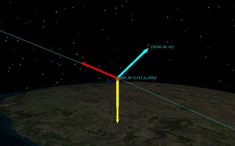
DMSP_5D-3_F17_D_29524 and vectors
Creating a report of magnetic vector components
Choose your data provider and create a custom report using the Report & Graph Manager.
- Right click on DMSP_5D-3_F17_D_29524 () in the Object Browser.
- Select Report & Graph Manager... (
 ).
). - Select the My Styles (
 ) folder in the Styles panel in the Report & Graph Manager.
 - Click Create new report style (
 ).
). - Type Magfield Vector to name your report.
- Press Enter on your keyboard to open the report's properties ().
Choosing a data provider
You will use the SEET Magnetic Field data provider. This data provider computes the geomagnetic field and various parameters associated with the geomagnetic field.
- Select the Content page in the Properties Browser ().
- Expand (
 ) SEET Magnetic Field in the data provider list.
 - Move (
 ) the following elements to the Report Contents list.
 - Time (
 )
) - B Field - ECF x ()
- B Field - ECF y ()
- B Field - ECF z ()
- Click .
- Select the Magfield Vector (
 ) report in the My Styles () folder.
 - Click .
- Close (
 ) the report when finished viewing the report.
 - Close () the Report & Graph Manager.
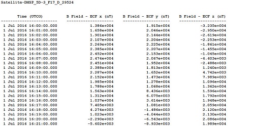
magfield vector report
Inserting Boston
- Insert a Place (
 ) object using the From City Database () method.
 - Type Boston in the Name: field in the Search Standard Object Data dialog box.
- Click .
- Select Boston Massachusetts in the Results: list.
- Click .
- Click to close the Search Standard Object Data dialog box when Boston () is added to the scenario.
Turning off Boston's Line of Sight constraint
You can turn off the Line of Sight constraint. The object will be able to create an access through the central body (e.g. the Earth).
- Open Boston's () properties ().
- Select the Constraints - Active page.
- Clear the Enable Line Of Sight check box.
- Click .
Setting DMSP_5D-3_F17_D_29524's constraints
Turning off the satellite's Ling of Sight constraint
First, turn off the Line of Sight constraint.
- Open DMSP_5D-3_F17_D_29524's () properties ().
- Select the Constraints - Active page.
- Clear the Enable Line Of Sight check box.
Adding the Magnetic Field Line Separation constraint
- Click Add new constraints (
 ) in the Active Constraints toolbar.
 - Select Magnetic Field Line Separation in the Constraint Name list in the Select Constraints to Add dialog box.
- Click .
- Click to close the Select Constraints to Add dialog box.
- Enter 0 deg in the Min: field located in the Magnetic Field Line Separation panel in the Constraint Properties section.
- Select the Max: check box.
- Enter 10 deg in the Max: field
- Click .
Setting STK SEET environment graphics
STK SEET can display magnetic-field contour lines for a Satellite (![]() ) object. The contour lines are displayed as field line footprint locations on the ground in the 2D Graphics window and as field-line maps in the 3D Graphics window.
) object. The contour lines are displayed as field line footprint locations on the ground in the 2D Graphics window and as field-line maps in the 3D Graphics window.
- Select the 2D Graphics - SEET Environment page.
- Select the Show 3D check box in the Magnetic Field Contour Line panel.
- Click .
Generating an access between DMSP_5D-3_F17_D_29524 and Boston
Create an access between DMSP_5D-3_F17_D_29524 (![]() ) and Boston (
) and Boston (![]() ).
).
- Right click on DMSP_5D-3_F17_D_29524 () in the Object Browser.
- Select Access... (
 ).
). - Select Boston () in the Associated Objects list.
- Click
 .
. - Click .
Generating an Access Intervals by Constraint report
This reports the intervals satisfying each constraint in the constraint set computed for the access, in the order in which the constraints were applied. You turned off line of sight for both objects and applied Magnetic Field Line Separation for DMSP_5D-3_F17_D_29524 (![]() ) . When the Magnetic Field Line Separation is small, this condition is known as magnetic conjugacy. The Access Intervals by Constraint (
) . When the Magnetic Field Line Separation is small, this condition is known as magnetic conjugacy. The Access Intervals by Constraint (![]() ) report tells you when this takes place in your scenario.
) report tells you when this takes place in your scenario.
- Select the Access Intervals by Constraint (
 ) report in the Installed Styles () list when the Report & Graph Manager opens.
 - Click .
- View the data in the report.
- Close () the report when finished.
Generating a geomagnetic conjugacy report
This report computes time intervals when DMSP_5D-3_F17_D_29524 (![]() ) is magnetically conjugate with Boston (
) is magnetically conjugate with Boston (![]() ).
).
- Return to the Report & Graph Manager.
- Select Satellite for the Object Type.
- Select DMSP_5D-3_F17_D_29524 () in the Object list.
- Select the SEET Geomagnetic Conjugacy () report in the Installed Styles () list.
- Click .
- Select Boston () in the Available Objects list in the Magnetic Conjugacy for DMSP_5D-3_F17_D_29524 dialog box.
- Keep the Max Separation of 10 deg.
- Click to close Magnetic Conjugacy for DMSP_5D-3_F17_D_29524 dialog box and generate the report.
- View the data in the report.
- Keep the report open.
Viewing the separation angle in the 3D Graphics window
You can use the report to set your animation time in the scenario.
- Right click on the first time in the report.
- Select Time in the shortcut menu.
- Select Set Animation Time in the next shortcut menu.
- Bring the 3D Graphics window to the front.
- Click Start () to animate your scenario.
- Notice the dotted line (e.g. possibly red) near your orbit as you watch the animation.
- Click Reset () when finished to reset your scenario.
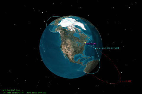
L-shell separation angle
This is the L-shell value showing the minimum to maximum angle separation.
Saving your work
- Close any open reports, properties and tools.
- Save () your work.
Summary
This was a quick introduction in using STK SEET. You inserted DMSP_5D-3_F17_D_29524 (![]() ) and Boston (
) and Boston (![]() ) into your scenario. You configured DMSP_5D-3_F17_D_29524 (
) into your scenario. You configured DMSP_5D-3_F17_D_29524 (![]() ) to use the IGRF magnetic field model. You turned off the line of site constraint for both DMSP_5D-3_F17_D_29524 (
) to use the IGRF magnetic field model. You turned off the line of site constraint for both DMSP_5D-3_F17_D_29524 (![]() ) and Boston (
) and Boston (![]() ) so that they could access each other through the central body (e.g. the Earth). You applied a magnetic field line separation constraint on DMSP_5D-3_F17_D_29524 (
) so that they could access each other through the central body (e.g. the Earth). You applied a magnetic field line separation constraint on DMSP_5D-3_F17_D_29524 (![]() ) . Finally, you created two reports, one showing when the intervals satisfying each constraint in the constraint set was computed for the access and the second computed time intervals when DMSP_5D-3_F17_D_29524 (
) . Finally, you created two reports, one showing when the intervals satisfying each constraint in the constraint set was computed for the access and the second computed time intervals when DMSP_5D-3_F17_D_29524 (![]() ) was magnetically conjugate with Boston (
) was magnetically conjugate with Boston (![]() ).
).