STK Pro, STK Premium (Air), STK Premium (Space), or STK Enterprise
You can obtain the necessary licenses for this tutorial by contacting AGI Support at support@agi.com or 1-800-924-7244.
This lesson requires STK 12.5 or newer to complete it in its entirety. It includes new features introduced in STK 12.5.
The results of the tutorial may vary depending on the user settings and data enabled (online operations, terrain server, dynamic Earth data, etc.). It is acceptable to have different results.
Capabilities covered
This lesson covers the following STK Capabilities:
- STK Pro
- Radar
- Coverage
Problem Statement
You need to forecast the capabilities of a synthetic aperture radar (SAR) that is attached to a satellite. The radar is shared by multiple agencies, and you are scheduled to use it during a 48-hour period. The satellite is in a circular orbit at an altitude of approximately 800 kilometers (km) above the Earth's surface. The SAR uses a small phased array antenna containing 16 elements. The elements have limited steering capability. The objective of the test is to determine if the radar can image the ground in a targeted region. If not, you might have to reschedule your 48-hour period to use the SAR.
Solution
Use STK's Pro, Radar and Coverage capabilities to analyze the SAR signal to noise ratio (SNR) in the target area. You will:
- Place the satellite in its orbit
- Build the SAR to specifications
- Use Coverage to determine SNR over the target area
What You Will Learn
Upon completion of this tutorial, you will be able to:
- Build a monostatic synthetic aperture radar (SAR)
- Use Coverage and the Figure Of Merit Access Constraint SAR signal-to-noise ratio (SarSNR)
Video Guidance
Watch the following video. Then follow the steps below, which incorporate the systems and missions you work on (sample inputs provided).
Creating a new scenario
First, you must create a new STK scenario and then build from there.
- Launch STK (
 ).
). - Click
 Create a Scenario in the Welcome to STK dialog box.
 - Enter the following in the STK: New Scenario Wizard:
- Click to accept your settings.
- Click Save (
 ) when the scenario loads. A folder with the same name as your scenario is created for you.
 - Verify the scenario name and location in the Save As window.
- Click .
| Option | Value |
|---|---|
| Name | STK_SAR |
| Location | Default |
| Start | 1 Jun 2024 19:00:00.000 UTCG |
| Stop | + 2 days |
Save often during this lesson!
Disabling Terrain Server
Terrain will not be used in your analysis, so you can turn off the Terrain Server.
- Right- click on STK_SAR (
 ) in the Object Browser.
 - Select Properties (
 ).
). - Select the Basic - Terrain page.
- Clear the Use terrain server for analysis check box.
- Click to accept the changes and close the Properties Browser.
Inserting a Satellite ( ) object
The Satellite (![]() ) object models the properties and behavior of a vehicle in orbit around a central body. Use the Orbit Wizard to change the Satellite (
) object models the properties and behavior of a vehicle in orbit around a central body. Use the Orbit Wizard to change the Satellite (![]() ) object's orbital parameters.
) object's orbital parameters.
- Select Satellite () in the Insert STK Objects tool.
- Select the Orbit Wizard (
 ) method.
 - Click .
- Set the following parameters when the Orbit Wizard opens:
- Click to accept your changes and to close the Orbit Wizard.
| Option | Value |
|---|---|
| Type | Circular |
| Satellite Name | SAR_Sat |
| Altitude | 800 km |
| RAAN | 220 deg |
Synthetic Aperture Radar (SAR)
A synthetic aperture radar achieves high resolution in the cross-range dimension by taking advantage of the motion of the vehicle carrying the radar to synthesize the effect of a large antenna aperture.
Inserting a Radar ( ) object
The Radar (![]() ) object will model the characteristics of a radar system and its environment.
) object will model the characteristics of a radar system and its environment.
- Insert a Radar () object using the Insert Default () method.
- Select SAR_Sat () in the Select Object dialog box.
- Click to close the Select Object dialog box.
- Right click on Radar1 () in the Object Browser.
- Select Rename in the shortcut menu.
- Rename Radar1 () to SAR_PhasedArray.
Modeling a SAR
Model the radar as SAR.
- Open SAR_PhasedArray's () properties ().
- Select the Basic - Definition page.
- Select the Mode tab.
- Click the Radar Monostatic Mode Component Selector (
 ).
). - Select SAR (
 ) in the Radar Monostatic Modes list in the Select Component dialog box.
 - Click to accept your selection and to close the Select Component dialog box.
Updaing SAR's Pulse Definition
Update the SAR's pulse definition. The satellite orbits at an approximate altitude of 800 kilometers. Range Resolution is a user-definable parameter inversely related to the pulse-compressed RF bandwidth of the transmitted signal.
- Select the Pulse Definition sub-tab.
- Select the Unambiguous Range option.
- Enter 800 km in the Unambiguous Range field.
- Enter 10 m in the Range Resolution field.
- Click to accept your changes and to keep the Properties Browser open.
Modeling SAR's Antenna
The SAR uses a phased array antenna. The phased array antenna model consists of many radiating elements. Each element is modeled as an isotropic pattern.
- Select the Antenna tab.
- Select the Model Specs sub-tab.
- Click the Antenna Model Component Selector ().
- Select Phased Array () in the Antenna Models list in the Select Component dialog box.
- Click to accept your selection and to close the Select Component dialog box.
Setting the Antenna's model specs
Set the design frequency and element configuration. The antenna design frequency is independent of the operational frequency of the radar. Element configuration enables you to define the physical aspects of the antenna elements.
- Enter 5 GHz in the Design Frequency: field.
- Select the Element Configuration sub-sub-tab.
- Set the following Designer parameters:
- Click to accept your changes and to keep the Properties Browser open.
| Option | Value |
|---|---|
| Type | Polygon |
| Lattice Structure - Type | Rectangular |
| Number of Elements - X | 5 |
| Number of Elements - Y | 4 |
Setting the Antenna's steering
The Beam Direction Provider enables you to select where the antenna points its beam. You have limited elevation steering for your antenna elements. The Auto Pointing Direction Provider will steer the antenna's beam toward the direction associated with the other Access object which will be the target grid that you will define later in your scenario.
- Select the Beam Direction Provider sub-sub-tab.
- Open the Type: drop-down list.
- Select Auto Pointing.
- Set the following Azimuth Steering parameters:
- Note that when steering limits are exceeded, Clamp-To-Limit is turned on. It causes the antenna to clamp the steering limit(s) when the object is outside Steering Limits.
- Click to accept your changes and to keep the Properties Browser open.
| Option | Values |
|---|---|
| Limit A | -25 deg |
| Limit B | 25 deg |
Setting the Transmitter's frequency and power
Set the transmitter's frequency and power.
- Select the Transmitter tab.
- Select the Specs sub-tab.
- Select the Frequency option.
- Set Frequency to 5 GHz.
- Set Power to 50 dBW.
- Click to accept your changes and to keep the Properties Browser open.
Modeling additional Gains and Losses
Use Post-Transmit Gains/Losses to define your gain. During radar analysis it is often necessary to model gains and losses that affect performance, but are not defined using built-in analytical models.
- Select the Additional Gains and Losses sub-tab.
- Click .
- Set Gain to 20 dB in the Post Transmit Gains/Losses section.
- Click to accept your changes and to keep the Properties Browser open.
Setting the Receiver's Gain
Set the Receiver's gain.
- Select the Receiver tab.
- Select the Additional Gains and Losses sub-tab.
- Click .
- Set Gain to 20 dB in the Pre-Receive Gains/Losses section.
- Click to accept your changes and to close the Properties Browser.
Coverage Definition
The Coverage Definition (![]() ) object defines a coverage area for analysis.
) object defines a coverage area for analysis.
Inserting a Coverage Definition
Insert a Coverage Definition (![]() ) into your scenario.
) into your scenario.
- Insert a Coverage Definition (
 ) object using the Insert Default () method.
 - Rename CoverageDefintion1 () to SAR_Cov.
Defining the Grid Area of Interest
LatLon Region creates a grid between the latitude and longitude point pairs you select.
- Open SAR_Cov's () properties ().
- Select the Basic - Grid page.
- Open the Type: drop-down list in the Grid Area of Interest panel.
- Select LatLon Region.
- Set the following:
- Click to accept your changes and to keep the Properties Browser open.
| Option | Value |
|---|---|
| Min. Latitude | 32.2412 deg |
| Min. Longitude | -121.936 deg |
| Max. Latitude | 38.0225 deg |
| Max. Longitutude | -117.244 deg |
Defining the Grid
The statistical data computed during a coverage analysis is based on a set of locations, or points, which span the specified grid area of interest. You can determine the spacing between the grid points using the Grid Definition options.
- Set Point Granularity - Lat/Lon to 0.1 deg.
- Click to accept your changes and to keep the Properties Browser open.
Setting the Coverage Assets
Assets properties enable you to specify the STK objects used to provide coverage.
- Select the Basic - Assets page.
- Expand (
 ) SAR_Sat () in the Assets list.
 - Select SAR_PhasedArrary ().
- Click .
- Click to accept your changes and to keep the Properties Browser open.
Turning off automatically recomputing Accesses
When Automatically Recompute Accesses is turned on, STK automatically recomputes assesses every time an object on which the coverage definition depends (such as an asset) is updated. Turning this option off allows you to manually recompute coverage when you are ready.
- Select the Basic - Advanced page.
- Clear Automatically Recompute Accesses.
- Click to accept your changes and to close the Properties Browser.
Computing Accesses
The ultimate goal of coverage is to analyze accesses to an area using assigned assets and applying necessary limitations upon those accesses. The Compute Accesses tool allows you to compute accesses between the grid points and the assigned assets.
STK's Parallel Computing capability enables STK to distribute many of its most computationally complex analysis tasks across multiple computing cores on the computer.
- Select SAR_Cov () in the Object Browser.
- Expand the CoverageDefinition menu.
- Select Compute Accesses in Parallel.
Figure of Merit Object
The Coverage Figure Of Merit (![]() ) object enables you to analyze coverage in various directions over time using several attitude-dependent figures of merit.
) object enables you to analyze coverage in various directions over time using several attitude-dependent figures of merit.
Inserting a Figure of Merit
Insert a Figure of Merit (![]() ) into your scenario.
) into your scenario.
- Insert a Figure Of Merit (
 ) object using the Insert Default () method.
 - Select SAR_Cov () in the Select Object dialog box.
- Click to close the Select Object dialog box.
- Rename FigureOfMerit1 () to SAR_SNR.
Setting Access Constraints
Your analysis requires you to measure an access constraint. Access Constraints measure the value of various constraint parameters used to define visibility within STK. The Access Constraint Figure of Merit reports the value of the selected access constraint definition at each grid point. SarSNR measures the signal-to-noise ratio for the SAR.
- Open SAR_SNR's () properties ().
- Select the Basic - Definition page.
- Set the following in the Definition panel:
- Click to accept your changes and to keep the Properties Browser open.
| Option | Value |
|---|---|
| Type | Access Constraint |
| Constraints | SarSNR |
| Compute | Maximum |
Analyzing the Grid
The Figure of Merit Overall Value data provider provides statistical information on static values. Statistics are generated by sampling values from all grid points. The Overall Value elements that you are interested in are Minimum (Minimum (dB)) and Maximum (Maximum (dB)). For your purposes, you require a SarSNR at or above 0 dB. The Grid Stats report provides this analysis.
- Right click on SAR_SNR () in the Object Browser.
- Select Report & Graph Manager... (
 ).
). - Select the Grid Stats (
 ) report in the Installed Styles (
 ) directory.
 - Click
- Scroll to the bottom of the report.
- Note that both the Minimum (dB) and Maximum (dB) values are above the required 0 dB.
- Keep the Grid Stats report open.
The minimum (dB) simply means that at least one point in your grid contains that value. The maximum (dB) means that at least one point in your grid contains that value.
Static Contours
The Figure of Merit's Static page enables you to define static graphics for your Figure Of Merit (![]() ) Object. Creating color contours is great for situational awareness and using a snapshot of the 2D and/or 3D Graphics window(s) can be used in a presentation.
) Object. Creating color contours is great for situational awareness and using a snapshot of the 2D and/or 3D Graphics window(s) can be used in a presentation.
Defining Static Graphics for the FOM
Define static graphics for the FOM.
- Return to SAR_SNR's () properties ().
- Select the 2D Graphics - Static page.
- Enter 30 in the % Translucency field in the Show Points As panel.
- Select the Show Contours option in the Display Metric panel.
- Set the following in the Level Adding section. You will use the rounded down minimum (dB) and maximum (dB) values from the Grid Stats report.
- Click .
- Ensure Color Method: is set at Color Ramp.
- Set the following:
- Select the following in the Contour Interpolation (points must be filled) section:
Option Natural Neighbor Show lines at level boundaries - Click to accept your changes and to keep the Properties Browser open.
| Option | Value |
|---|---|
| Start | 0 dB |
| Stop | 55 dB |
| Step: | 5 dB |
| Option | Value |
|---|---|
| Start Color | Red |
| End Color | Blue |
Show lines at level boundaries displays contour lines for all the specified contour levels. It's another way to enhance your contours.
Displaying Contour Legends
The Legend provides you with a convenient way to interpret contour data displayed in the 2D and 3D Graphics windows. You can set the display of the Contours Legend by opening the Contours Legend Layout window.
- Click in the Level Attributes panel.
- Click in the Static Legend for SAR_SNR floating legend.
- Set the following on the figure of Merit Legend Layout dialog box:
Option Value 2D Graphics Window - Show at Pixel Location Select 3D Graphics Window - Show at Pixel Location Select Text Options - Title Signal to Noise Ratio (dB) Text Options - Number Of Decimal Digits 0 Range Color Options - Color Square Width (pixels) 50 - Click to accept your changes and to close the Figure of Merit Legend Layout dialog box.
- Close (
 ) the Static Legend for SAR_SNR floating legend.
 - Click to accept your changes and to close the Properties Browser.
Viewing Contours
You can view the static contours in both the 2D and 3D Graphics windows.
- Bring the 2D Graphics window to the front.
- Use your mouse to center on and zoom in on your coverage grid.
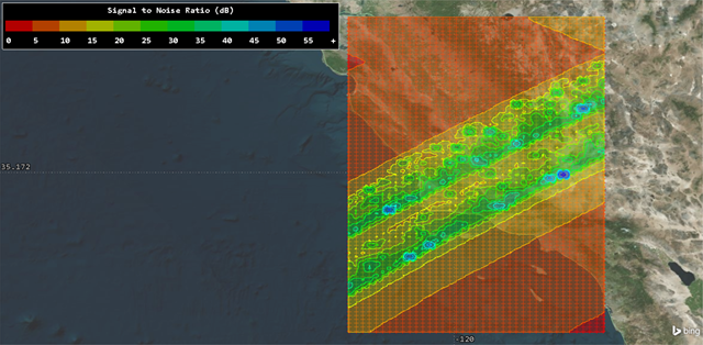
SAR SNR Contours
Saving Your Work
Save your work when you are finished.
- Close any properties, reports, or tools that are still open.
- Save () your work.
Summary
You used STK to determine if your scheduled time using a synthetic aperture radar (SAR) on a LEO satellite would produce acceptable values needed to perform mapping of a target grid. You placed the satellite into its orbit and built a SAR to specifications. You used Coverage to create the target grid and selected the SAR as your asset. After computing coverage accesses using parallel computing, you inserted a Figure of Merit (FOM) which allowed you to focus on SAR signal-to-noise ratio inside the grid. You demonstrated that during your scheduled time the SAR on a LEO satellite is able to access grid points in a target area and receive an acceptable reflection based on a signal to noise ratio of 0 dB or higher.