STK Pro, STK Premium (Air), STK Premium (Space), or STK Enterprise
You can obtain the necessary licenses for this tutorial by contacting AGI Support at support@agi.com or 1-800-924-7244.
The results of the tutorial may vary depending on the user settings and data enabled (online operations, terrain server, dynamic Earth data, etc.). It is acceptable to have different results.
This lesson requires an Internet connection and version 12.8 of the STK software or newer to complete.
Capabilities covered
This lesson covers the following capabilities of the Ansys Systems Tool Kit® (STK®) digital mission engineering software:
- STK Pro
- Communications
Problem statement
Engineers and operators require a quick and simple way to simulate and analyze multi-hop communications links. A ship passing through the Panama Canal needs to transmit data to another ship located in the Strait of Hormuz by way of two satellites in geosynchronous orbit. The entire communications system is analog. The surface units are using K-Band communications in the 18-24 GHz range; satellite-to-satellite communications are via the S-Band in the 2-4 GHz range. The ship transiting the Panama Canal can target its phased array antennas at the satellite; satellite-to-satellite communications are also targeted via small parabolic and Gaussian antennas. The satellite-to-surface antennas are fixed and boresighted towards the Panama Canal and the Strait of Hormuz. The ship transiting the Strait of Hormuz can target its parabolic receiver antenna at the satellite. You are looking for an opportunity during which you can pass data between the two ships.
Solution
Use the STK software's Communications capability to model a scenario that analyzes a multi-hop communications link from the ship transiting the Panama Canal to a ship transiting the Strait of Hormuz. Apply the STK application's radio frequency environmental features to perform a realistic communications analysis.
What you will learn
Upon completion of this tutorial, you will understand:
- How to model multi-hop communications involving analog transponders
- How to enable rain and atmospheric absorption models for communications analysis
- How to generate a custom Bent Pipe Comm Link report using the Chain object and the Report & Graph Manager
Video guidance
Watch the following video. Then follow the steps below, which incorporate the systems and missions you work on (sample inputs provided).
Using a starter scenario (*vdf file)
To speed things up and allow you to focus on the portion of this exercise that teaches you build a multi-hop communications system in the STK application, a partially created scenario has been provided for you.
- Launch the STK application (
 ).
). - Click (
 ) in the Open dialog box.
 - Browse to <Install Dir>\Data\Resources\stktraining\VDFs.
- Select Comm_MultiHopLink.vdf.
- Click .
Saving a VDF as a scenario file
When you save a scenario in the STK application, it will save in the format in which it originated. In other words, if you open a VDF, the default save format will be a VDF (.vdf). The same is true for a scenario file (*.sc). If you want to save a VDF as a SC file (or vice-versa), you must change the file format when you are performing the Save As procedure.
- Open the File menu.
- Select Save As....
- Select the STK User folder in the navigation pane.
- Select Comm_MultiHopLink (
 ).
). - Click .
- Open the Save as type drop-down list.
- Select Scenario Files (*.sc).
- Click .
- Click to Replace existing file.
When saving a VDF as a scenario folder, you should extract its contents to the scenario folder the STK application automatically creates for you in the STK User folder. See the
Save (![]() ) your scenario often!
) your scenario often!
Reviewing the starter scenario
Prior to beginning the scenario, you can get an overall feel of where each object is located and where the different sensors point.
- Bring the 2D Graphics window to the front.
- Review the placement of the ships, sensors, and satellites.
- Bring the 3D Graphics window to the front.
A communications link exists between Canal_Transit and Geo_West. Canal_Transit is transmitting on a frequency of 20 GHz with a power of 30 dBW. Canal_Transit is transmitting via a phased array antenna. Geo_West is using a 4.6-meter diameter fixed-boresight parabolic receiver antenna.
In the Object Browser, you can see there are multiple Sensor objects. The Sensor objects are simulating servo motors and are being used to point steerable antennas at specific targets or to boresight an antenna at a specific area.
Note the satellite’s sensor boresight contour over the Panama Canal.
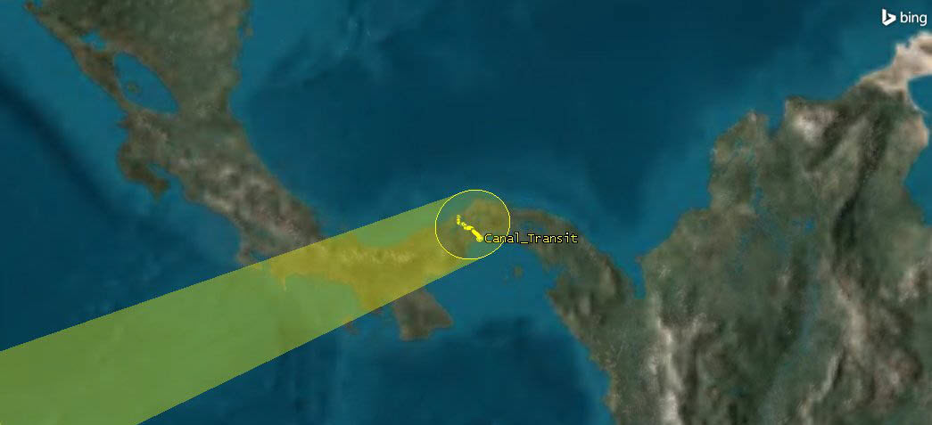
Panama Canal boresight
Configuring the scenario rain loss and atmospheric models
Loading the ITU-R rain loss model
When enabled, you can use a
You will use the
- Right-click on Comm_MultiHopLink (
 ) in the Object Browser.
 - Select Properties (
 ).
). - Select the RF - Environment page when the Properties Browser opens.
- Select the Rain, Cloud & Fog tab.
- Select the Use check box in the Rain Model panel.
- Click the Rain Loss Model Component Selector (
 ).
). - Select the newest ITU-R (International Telecommunication Union) model — for example, ITU-R P618-13 (
 ) — in the Rain Loss Models list when the Select Component dialog box opens.
 - Click to close the Select Component dialog box.
- Click to accept the changes and keep the Properties Browser open.
This will open the
Loading the ITU-R atmospheric absorption model
You will use the
- Select the Atmospheric Absorption tab.
- Select the Use check box.
- Click the Atmospheric Absorption Model Component Selector ().
- Select the newest ITU-R (International Telecommunication Union) model — for example, ITU-R P676-13 () — in the Atmospheric Absorption Models list when the Select Component dialog box opens.
- Click to close the Select Component dialog box.
- Click to accept your changes and to close the Properties Browser.
Building the transmission uplink from the Panama Canal
You'll build the communications link starting where the transmission begins at the Panama Canal and follow the transmission until it reaches its destination. You will attach a Transmitter or Receiver object to a specified Sensor object, which will point the embedded antenna at a target.
Inserting Canal_Transit's uplink transmitter
Create a new Transmitter object and attach it to the ship transiting the Panama Canal. A
- Select Transmitter (
 ) in the Insert STK Objects tool.
 - Select the Insert Default () method.
- Click .
- Select Canal_Transit (
 ) in the Select Object dialog box.
 - Click .
- Right-click on Transmitter1 () in the Object Browser.
- Select Rename in the shortcut menu.
- Rename Transmitter1 () UplinkXmtr.
Selecting a Complex Transmitter Model
A
- Open UplinkXmtr's () Properties ().
- Select the Basic - Definition page when the Properties Browser opens.
- Click the Transmitter Model Component Selector ().
- Select Complex Transmitter Model () in the Transmitter Models list when the Select Component dialog box opens.
- Click to close the Select Component dialog box.
- Select the Model Specs tab.
- Enter 20 GHz in the Frequency field.
- Enter 8 Mb/sec in the Data Rate field.
- Click to accept your changes and to keep the Properties Browser open.
Modeling a phased array antenna
A
- Select the Antenna tab.
- Click the Antenna Model Component Selector ().
- Select Phased Array () in the Antenna Models list when the Select Component dialog box opens.
- Click to close the Select Component dialog box.
- Select the Model Specs sub tab.
- Enter 21 GHz in the Design Frequency field.
Configuring the antenna elements
The
- Select the Element Configuration sub-sub tab.
- Enter the following in the Number of Elements panel:
- Click to accept your changes and to keep the Properties Browser open.
| Option | Value |
|---|---|
| X | 7 |
| Y | 7 |
Selecting the beam direction provider
The
- Select the Beam Direction Provider sub-sub tab.
- Select the Enabled check box in the Beam Steering panel.
- Move (
 ) Geo_West (
 ) from the objects list to the selected objects list.
 - Click to accept your changes and to keep the Properties Browser open.
Orienting the antenna
The STK application provides
- Select the Orientation sub tab.
- Set the following in the Position Offset panel:
- Click to accept your changes and to keep the Properties Browser open.
| Option | Value |
|---|---|
| X | -42 m |
| Y | -29 m |
| Z | 35 m |
Displaying the antenna pattern in the 3D Graphics window
The
- Select the 3D Graphics - Attributes page.
- Select the Show Volume check box in the Volume Graphics panel.
- Enter the following settings:
- Select the Set azimuth and elevation resolution together check box in the Pattern panel.
- Click to accept your changes and to close the Properties Browser.
| Option | Value |
|---|---|
| Show as wireframe | Selected |
| Gain Scale (per dB) | 0.1 km |
| Minimum Displayed Gain | -5 dB |
You can use these steps later in the lesson to view other antenna patterns if you desire to do so.
Viewing the antenna pattern in the 3D Graphics window
View Canal_Transit's antenna pattern in the 3D Graphics window.
- Bring the 3D Graphics window to the front.
- Right-click on Canal_Transit () in the Object Browser.
- Select Zoom To.
- Use your mouse to zoom out so that you can see the phased array antenna pattern.
- Notice that the antenna pattern is located on the ship's superstructure where the actual antenna is located on the ship.
![]()
Canal_Transit's phased array antenna pattern
Creating the first analog transponder
In an analog transponder, the transmitted signal is essentially a reflection of the received signal, with the added possibility of frequency translation or power amplification. You'll begin modeling the analog transponder on the Geo_West satellite with a Receiver object attached to the TgtCanalZone Sensor object.
Creating a new receiver
A
- Insert a Receiver (
 ) object using the Insert Default () method.
 - Select TgtCanalZone (
 ) in the Select Object dialog box.
 - Click to close the Select Object dialog box.
- Rename Receiver1 () UplinkRcvr.
Using a Complex Receiver model
A
- Open UplinkRcvr's () Properties ().
- Select the Basic - Definition page when the Properties Browser opens.
- Click the Receiver Model Component Selector ().
- Select Complex Receiver Model () in the Receiver Models list when the Select Component dialog box opens.
- Click to close the Select Component dialog box.
- Click to accept your change and to keep the Properties Browser open.
Modeling a parabolic antenna
A
- Select the Antenna tab.
- Select the Model Specs sub tab.
- Click the Antenna Model Component Selector ().
- Select the Parabolic () in the Antenna Models list when the Select Component dialog box opens.
- Click to close the Select Component dialog box.
- Enter 21 GHz in the Design Frequency field.
- Enter 4.6 m in the Diameter field.
- Click to accept your changes and to keep the Properties Browser open.
Adding additional gains and losses
During communications analyses, it is often necessary to model
- Select the Additional Gains and Losses tab.
- Click Add in the Pre-Receive Gains/Losses panel.
- Enter 2 dB in the Gain cell.
- Click Add in the Pre-Demodulation Gains/Losses panel.
- Enter 2 dB in the Gain cell.
- Click to accept your changes and to close the Properties Browser.
Creating a new Transmitter object
Attach a Transmitter object to the Tgt_Geo_East Sensor object for the second half of the transponder.
- Insert a Transmitter () object using the Insert Default () method.
- Select Tgt_Geo_East () in the Select Object dialog box.
- Click to close the Select Object dialog box.
- Rename Transmitter2 () Geo_West_ReXmtr.
Using a Complex Retransmitter model
A
- Open Geo_West_ReXmtr 's () Properties ().
- Select the Basic - Definition page when the Properties Browser opens.
- Click the Transmitter Model Component Selector ().
- Select Complex Re-Transmitter Model () in the Transmitter Models list when the Select Component dialog box opens.
- Click to close the Select Component dialog box.
- Select the Model Specs tab.
- Set the following parameters:
- Click to accept your changes and to keep the Properties Browser open.
| Option | Value |
|---|---|
| Sat. Power | 20 dBW |
| Sat. Flux Density | -120 dBW/m^2 |
Sat. Power or Saturation Output Power is the RF Power output of the transmitter as measured at the input to the antenna when the amplifier is at its saturated state.
Sat. Flux Density or Saturation Flux Density (SFD) is the amplifier's saturation point by the input flux density in dBW/m2. This represents the per carrier flux density for systems supporting multiple carriers per transmitter. A lower SFD value makes the input of the transponder more sensitive and requires less uplink power from the uplink station. Increasing the sensitivity in the transponder allows the introduction of more noise into the system, due to the higher sensitivity.
Selecting a Gaussian Antenna model
A
- Select the Antenna tab.
- Keep the Gaussian Antenna Model type.
- Enter 3 GHz in the Design Frequency field.
- Enter 2 m in the Diameter field.
- Click to accept your changes and to keep the Properties Browser open.
Setting the transfer function frequency coefficients
Frequency coefficients specify the transmitted frequency as a function of the received frequency. They can only be entered in polynomial form. The coefficient order displays in the left column of the table and updates automatically as coefficients are added or removed. Input and output units are in Hz. The default coefficients of -7.0e+08 and 1.0 are used to model a 700 MHz down conversion. The transmitter is transmitting on a frequency of 4 GHz.
- Select the Transfer Functions tab.
- Change the Index 0 Coefficient to -1.6e+010.
- Click to accept your changes and to close the Properties Browser.
Creating the second analog transponder
Next, model the transponder on board the Geo_East satellite.
Reusing UplinkRcvr
Continue building the link by attaching a Receiver object to the Geo_East satellite. You can simplify this process by reusing the UplinkRcvr Receiver object. from the Geo_West satellite and then updating its properties.
- Select UplinkRcvr () in the Object Browser.
- Click Copy (
 ) in the Object Browser toolbar.
 - Select Tgt_Geo_West () in the Object Browser.
- Click Paste (
 ) in the Object Browser toolbar.
 - Rename UplinkRcvr1 () Geo_East_Rcvr.
Updating the receiver's properties
You need to make a couple of changes to Geo_East_Rcvr's properties.
- Open Geo_East_Rcvr's () Properties ().
- Select the Basic - Definition page when the Properties Browser opens.
- Select the Antenna tab.
- Set the Design Frequency to 3 GHz.
- Enter 2 m in the Diameter field.
- Click to accept your changes and to close the Properties Browser.
Reusing Geo_West_ReXmtr
The Geo_East satellite will retransmit the data to Hormuz_Transit.
- Copy () Geo_West_ReXmtr () and paste () it on TgtHormuz () in the Object Browser.
- Rename Geo_West_ReXmtr1 () Geo_East_ReXmtr.
Changing the antenna's properties
Configure a Parabolic Antenna model for the Geo_East_ReXmt transmitter.
- Open Geo_East_ReXmtr's () Properties ().
- Select the Basic - Definition page when the Properties Browser opens.
- Select the Antenna tab.
- Select the Model Specs sub-tab.
- Click the Antenna Model Component Selector ().
- Select Parabolic () in the Antenna Models list when the Select Component dialog box opens.
- Click to close the Select Component dialog box.
- Enter 21 GHz in the Design Frequency field.
- Enter 4.6 m in the Diameter field.
- Click to accept your changes and to keep the Properties Browser open.
Setting the transfer function frequency coefficients
The downlink frequency is 18 GHz.
- Select the Transfer Functions tab.
- Change the Index 0 Coefficient to 1.4e+10.
- Click to accept your changes and to close the Properties Browser.
Creating the transmission downlink at the Strait of Hormuz
The receiver on the Hormuz_Transit Ship object completes the communications link.
Reusing Geo_East_Rcvr
You can adapt the receiver from the Geo_East satellite for use with the sensor on Hormuz_Transit.
- Select Geo_East_Rcvr () in the Object Browser.
- Click Copy () in the Object Browser toolbar.
- Select TgtEastSat () in the Object Browser.
- Click Paste () in the Object Browser toolbar.
- Rename Geo_East_Rcvr1 () DownlinkRcvr.
Changing the antenna properties
Configure DownlinkRcvr's design frequency and antenna diameter.
- Open DownlinkRcvr's () Properties ().
- Select the Basic - Definition page when the Properties Browser opens.
- Select the Antenna tab.
- Enter 21 GHz in the Design Frequency field.
- Enter 3 m in the Diameter field.
- Click to accept your changes and to close the Properties Browser.
Creating a Chain object
A
Adding a new Chain object
Create a Chain object that starts at UplinkXmtr and ends at DownlinkRcvr.
- Insert a Chain (
 ) object using the Insert Default () method.
 - Rename Chain1 () AnalogLink.
Defining the start and end objects
Start by choosing the start object and end object in your chain.
- Open AnalogLink's () Properties ().
- Select the Basic - Definition page when the Properties Browser opens.
- Click the Start Object ellipsis ().
- Select UplinkXmtr () in the Select Object dialog box.
- Click to close the Select Object dialog box.
- Click the End Object ellipsis ().
- Select DownlinkRcvr () in the Select Object dialog box.
- Click to close the Select Object dialog box.
Creating the Chain object's connections
After you choose the start and end objects in your chain, you need to build the chain's connections. It doesn't matter in which order you place the connections in the Connections list. What matters is the From Object must be able to access the To Object.
Building the first connection
Build your first connection from UplinkXmtr to UplinkRcvr.
- Click in the Connections panel.
- Click the From Object ellipsis ().
- Select UplinkXmtr () in the Select Object dialog box.
- Click to close the Select Object dialog box.
- Click the To Object ellipsis ().
- Select UplinkRcvr () in the Select Object dialog box.
- Click to close the Select Object dialog box.
Building the second connection
Extend the connection from UplinkRcvr to Geo_West_ReXmtr.
- Click .
- Click the To Object ellipsis ().
- Select Geo_West_ReXmtr () in the Select Object dialog box.
- Click to close the Select Object dialog box.
Building the third connection
Extend the connection from Geo_West_ReXmtr to Geo_East_Rcvr.
- Click .
- Click the To Object ellipsis ().
- Select Geo_East_Rcvr () in the Select Object dialog box.
- Click to close the Select Object dialog box.
Building the fourth connection
Extend the connection from Geo_East_Rcvr to Geo_East_ReXmtr.
- Click .
- Click the To Object ellipsis ().
- Select Geo_East_ReXmtr () in the Select Object dialog box.
- Click to close the Select Object dialog box.
Building the fifth and final connection
Finally, extend the connection from Geo_East_ReXmtr to DownlinkRcvr.
- Click .
- Click the To Object ellipsis ().
- Select DownlinkRcvr () in the Select Object dialog box.
- Click to close the Select Object dialog box.
- Click to accept your changes and to close the Properties Browser.
Viewing the communications link in the 2D Graphics window
You can see the completed link from Canal_Transit to Hormuz_Transit in the 2D Graphics window.
- Bring the 2D Graphics window to the front.
- Zoom out so that you can see the Panama Canal, both satellites and the Strait of Hormuz.
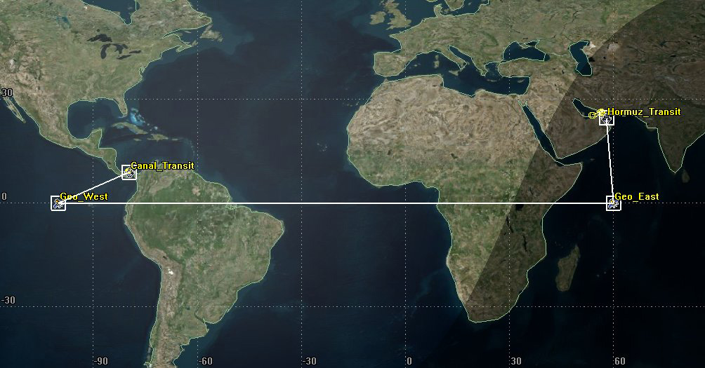
2D Completed Link
You should now see the completed communications link.
Creating a custom Bent Pipe Comm Link report
There are many parameters that reflect the quality of a signal, but the Bit Error Rate (BER) is typically a good indicator. For this tutorial, you will focus on BER. The lower the BER, the better the quality of the signal. You can use a
By default, the STK application only handles two links in Bent Pipe Comm Link reports. This means you will have to create a unique report that will model the full communications link from Canal_Transit to Hormuz_Transit. You need to show the BER total for all three links by customizing the Bent Pipe Comm Link report in the Report & Graph Manager.
Copying the existing Bent Pipe Comm Link report
Duplicate the existing Bent Pipe Comm Link report so you can customize it for your needs.
- Right-click on AnalogLink () in the Object Browser.
- Select Report & Graph Manager... (
 ) in the shortcut menu.
 - Right-click on the Bent Pipe Comm Link (
 ) report in the Installed Styles () folder when the Report & Graph Manager opens.
 - Select Duplicate (
 ).
).
Selecting the data providers and elements
You create a new line in the report for additional data providers.
- Select the Content page when the Properties Browser opens.
- Select Link Information-BER2 in the Report Contents list.
- Click .
- Select Line 3 in the Report Contents list.
- Expand the Link Information () data provider in the Data Providers list.
- Add the following data provider elements (
 ) to Line 3 in the Report Contents list in the order shown:
 - Xmtr Power3
- Xmtr Gain3
- EIRP3
- Prop Loss3
- Rcvd. Frequency3
- Rcvd. Iso. Power3
- Flux Density3
- g/T3
- C/No3
- Bandwidth3
- C/N3
- Eb/No3
- BER3
Changing the report values to scientific notation
Changing the BER to scientific notation allows you to look at the significant digits and the exponent of 10, which is what is shown on the other BER lines.
- Select Link Information-BER3 in the Report Contents list.
- Click .
- Open the Notation drop-down list when the Options: Section 1, Line 3, Link Information-BER3 dialog box opens.
- Select Scientific (e).
- Click to close the Options: Section 1, Line 3, Link Information-BER3 dialog box.
Adding a line for the composite values
Add a new line that will show the composite values of the entire communications link.
- Select Line 4 in the Report Contents window.
- Click .
- Select Link Information-BER3.
- Click .
- You are still using the Link Information () data provider.
- Select Line 4.
- Add the following data provider elements () to Line 4 in the Report Contents list in the order shown:
- IBO3
- OBO3
- C/No Tot.3
- C/N Tot.3
- Eb/No Tot.3
- BER Tot.3
Setting the report value to scientific notation
As with BER3, changing BER Tot.3 to use scientific notation allows you to look at the significant digits and the exponent of 10.
- Select Link Information-BER Tot.3 in the Report Contents list.
- Click .
- Open the Notation drop-down list when the Options: Section 1, Line 3, Link Information-BER Tot.3 dialog box opens.
- Select Scientific (e).
- Click to close the Options: Section 1, Line 3, Link Information-BER Tot.3 dialog box.
- Click to accept your changes and to close the Properties Browser.
Generating your custom Bent Pipe Comm Link report
Your custom report has been moved to the My Styles (![]() ) folder. Rename it, then generate the report.
) folder. Rename it, then generate the report.
- Expand (
 ) the My Styles () folder in the Styles list.
 - Right-click on Bent Pipe Comm Link (
 ) in the My Styles () folder.
 - Select Rename in the shortcut menu.
- Rename Bent Pipe Comm Link () Analog Link.
- Click .
- In order to have a successful transmission, you are looking for a BER Tot.3 of 1.0e-10 or lower. While looking at the composite BERs, scroll through the report.
- Are there any fluctuations in the values?
- What is the time window when data can be transmitted successfully across the link?
Look at the first four lines in the report. The report contains link performance data for the uplink from Canal_Transit to Geo_West (first line), the link from Geo_West to Geo_East (second line), the link from Geo_East to Hormuz_Transit (third line), and the combined link (fourth line). Degradation in retransmitted signal and the composite link performance can readily be perceived by comparing BER1, BER2, and BER3 to BER Tot.3.
Notice the received frequencies for all the links to see how the transfer functions worked.
Saving your work
You can clean up and finish your scenario.
- Close any open reports, properties, and the Report & Graph Manager.
- Save (
 ) your work.
Summary
In this tutorial, you learned how to create a multi-hop analog transmission from a ship passing through the Panama Canal to a ship in the Strait of Hormuz via two satellites in geosynchronous orbit. The ship traveling through the Panama Canal deployed a phased array antenna and transmitted on a frequency of 20 GHz to a satellite named Geo_West. The analog transponder on Geo West retransmitted the signal using a Gaussian antenna on a frequency of 4 GHz to a satellite named Geo East. The analog transponder on the Geo_East satellite retransmitted the signal using a parabolic antenna on a frequency of 18 GHz to the ship in the Strait of Hormuz. You created a custom Bent Pipe Comm Link report to determine the time window during which you could be certain of transmitting information.
On your own
You can adjust power and data rates to see what effect the different combinations have on the custom Bent Pipe Comm Link report. For instance, you could decrease power and data rate and review the results.