STK Premium (Space), or STK Enterprise
You can obtain the necessary licenses for this tutorial by contacting AGI Support at support@agi.com or 1-800-924-7244.
Required product install: A 64-bit version of Java is required to run Analyzer. See the Analyzer system requirements for more information.
The results of the tutorial may vary depending on the user settings and data enabled (online operations, terrain server, dynamic Earth data, etc.). It is acceptable to have different results.
Capabilities covered
This lesson covers the following capabilities:
- STK Pro
- STK Analyzer
- Coverage
- Astrogator
Tutorial purpose
The following tutorial is designed to teach you how to use STK's Analyzer capability with STK's Astrogator capability. A basic knowledge of Astrogator is assumed. Should you require training in Astrogator prior to this tutorial, see our Level 2 - Advanced Training and Level 3 - Focused / Feature Specific Astrogator tutorials.
This tutorial consists of three exercises. Each exercise comes with a previously created scenario that was saved as a Visual Data (VDF) File.
- Exercise One: Compute the minimum thrust required to raise perigee.
- Exercise Two: Determine possible orbits that may result after small launch errors.
- Exercise Three: Minimize the amount of fuel used during a lunar mission.
Analyzer
Analyzer is integrated into the STK work flow to help you automate and analyze STK trade studies to better understand the design of your system. For purposes of this tutorial, you will use Analyzer to:
- Parametrically explore the STK design space to analyze various satellite orbital inputs.
- Perform parameter studies that vary an input variable through a range of values and plot one or more output variables.
Video Guidance
Watch the following video. Then follow the steps below, which incorporate the systems and missions you work on (sample inputs provided).Please note, the video refers to a starter scenario accessed from the STK Data Federate (SDF). This scenario is included with your STK install. Please follow the written steps in this tutorial to open the file.
Exercise One: Minimize Delta-V
The goal of Exercise One is to raise the perigee radius of a satellite to 10000 kilometers (km) using a single burn. As with most satellite applications, minimizing the amount of fuel used for maneuvers is of great concern. In this exercise, you want to minimize the change in Delta-V (velocity), since the minimum Delta-V will result in the least amount of fuel used.
First, use Analyzer’s Parametric Study to determine at which true anomaly this maneuver should be performed in order to minimize Delta-V. In this case, thrust will be fixed in the velocity direction.
Next, change the direction of thrust (azimuth and elevation) to see if this further minimizes the Delta-V required. This study will be performed using Analyzer’s Optimization Tool.
Using a starter scenario
To speed things up and have you to focus on the portion of this exercise that teaches you Analyzer, a partially created scenario has been provided for you.
Loading the starter scenario
The STK scenario (VDF) used with this tutorial is included with the STK installation. To open the scenario:
- Launch the STK® (
 ) application.
 - Click
 Open a Scenario in the Welcome to STK dialog.
 - Select Installed Scenarios in the navigation pane or browse to <STK install folder>\Data\ExampleScenarios.
Opening the VDF
- Select Analyzer_OptimumTrueAnamoly.vdf.
- Click .
Saving the starter scenario as an SC file
When you open the scenario, the STK application will create a folder with the same name as the scenario in the default user folder (C:\Users\<username>\Documents\STK_ODTK 13, for example). The STK application will not save the scenario automatically. When you choose save a scenario, the STK application will default to saving it in the format in which it originated. Therefore, if you open a VDF, the default save format will be a VDF. The same is true for a scenario file (*.sc). To save the VDF as an SC file, change the file format using the Save As procedure:
- Open the File menu.
- Select Save As....
- Select the STK User folder in the navigation pane when the Save As dialog box opens.
- Select the folder with the same name as the scenario.
- Click .
- Select Scenario Files (*.sc) in the Save as type drop-down list.
- Select the Scenario file in the file browser.
- Click .
- Click in the Confirm Save As Dialog box to overwrite the existing scenario file in the folder and to save your scenario.
A scenario folder with the same name as the VDF was created for you when you opened the VDF in the STK application. This folder contains the temporarily unpacked files from the VDF.
Reviewing the Satellite segments
Familiarize yourself with the orbital parameters of the satellite.
- Right-click Satellite (
 ) in the Object Browser and select Properties (
 ).
). - On the Basic - Orbit page, go to the Mission Control Sequence (MCS).
- Select the Initial State (
 ) Segment. Note the Elements.
Mission Control Sequence (MCS)
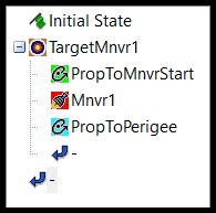
Reviewing the Target Sequence: TargetMnvr1
The satellite’s orbit is propagated until it reaches a true anomaly of 180 degrees — you will vary this value later in Analyzer — using a Target (![]() ) sequence.
) sequence.
- Select the Propagate (
 ) segment named PropToMnvrStart (
 ).
). - Select the Maneuver (
 ) segment named Mnvr1 (
 ).
). - Select the Propagate () segment named PropToPerigee (
 ).
). - At the bottom of the MCS, click .
- In the Multi-Component Select Window, R Mag is the selected result.
- Close the Multi-Component Select Window.
Note the Stopping Condition and Trip time.
Note the Attitude Control and other settings.
Note the stopping condition.
Seeing the Differential Corrector
A Differential Corrector Profile runs the Target (![]() ) sequence.
) sequence.
- Select TargetMnvr1 (
 ).
). - Click the Profile Properties () icon.
- Close (
 ) the Targeting Profile window.
The control parameter was originally set at 1200 seconds (set in Mnvr1 - Propagator). Equality Constraints desired result was set at 10000 km. To reach the desired result, Astrogator changed the control parameter. The orbit was then propagated until it reached Periapsis (perigee).
Creating a dependent variable for Analyzer
Since you are trying to vary true anomaly and determine its effect on Delta-V, true anomaly is the independent variable and Delta-V the dependent variable. To make Delta-V available as a variable, you need to select it as a result for the maneuver segment.
- In the MCS, select Mnvr1 (
 ).
). - At the bottom of the MCS, click .
- In the Available list, expand (
 ) Maneuver (
 ).
). - Select DeltaV (
 ).
). - Click the Insert Component right arrow (
 ).
). - Click to close the User-Selected Results window.
- Click to close Satellite's () properties.
Opening Analyzer
Click the Analyzer button on the Analyzer Tool Bar.

Analyzer Toolbar
Viewing the Analyzer layout
Use the Analyzer Main Form to configure input/output variables available for further analysis. You can first select an object in the scenario tree on the left. When you select an object, Analyzer lists all possible input variable candidates under the Inputs General tab and the Inputs Constraints tab. Analyzer lists all output variable candidates under the Outputs Data Providers tab, Outputs Object Coverage tab, Outputs DeckAccess tab, or Outputs MissileModelingTools tab.
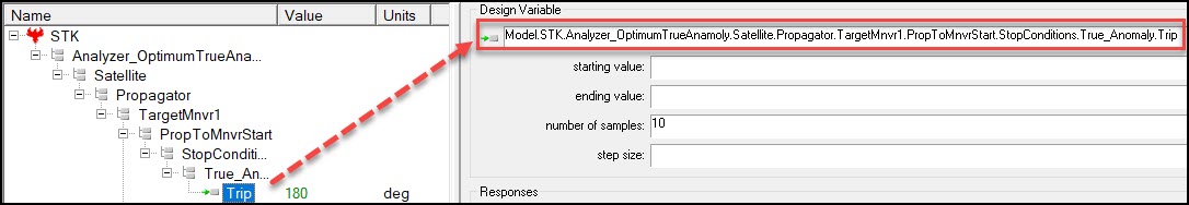
Setting the Input Variable
- In the STK Variables field, select Satellite ().
- In the STK Property Variables field, expand (
 ) the following in the order as shown:
 - Propagator (Astrogator) ()
- TargetMnvr1 (
 )
) - PropToMnvrStart ()
- StopConditions ()
- True_Anomaly ()
- Double-click Trip (
 ) to move it to the Analyzer Variables field.
Setting the Output Variable
- Return to TargetMnvr1 ().
- Expand () Mnvr1 ().
- Expand () Results ()
- Double-click the DeltaV () to move it to the Analyzer Variables field.

Using the Parametric Study Tool
The Parametric Study Tool runs a scenario through a sweep of values for some input variable. You can plot the resulting data to view trends.
- In the Analyzer tool bar, select Parametric Study.
- In the Component Tree, using your left mouse button, drag Trip (
 )to the Design Variable field on the right.
 - Set the following design values:
- In the Component Tree, using your left mouse button, drag DeltaV (
 ) to the Responses field on the right.
 - In the lower-right corner of the Parametric Study Tool, click .

Analyzer Toolbar and Parametric Study Icon
Another way of opening Analyzer is to go to the Object Browser, right-click the scenario object (or any object), select <Object> Plugins, and click Analyzer ( ).
).
Analyzer builds a parametric representation of the currently loaded Scenario. This representation appears in the Component Tree displayed on the left side of each trade study tool.
Drag and Drop Design Variable
| Option | Value |
|---|---|
| starting value | 160 |
| ending value | 180 |
| number of samples | 21 |
| step size | 1 |
Setting the step size will determine number of samples, which is the number of times the scenario changes in STK. Conversely, setting number of samples will determine step size.
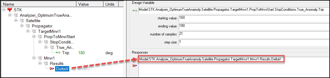
Drag and Drop Result
Using the Data Explorer
The Data Explorer is a tool used by Trade Study tools to display data while they are being collected from STK. While data is being collected, the Data Explorer displays a progress meter, a halt button, and the data.
Viewing the Table Page
The Table page displays trade study data in a tabular form. It is the default window that is present for all trade studies. Cells are shaded differently depending on the associated variable's state. Input variables are shown with green text, valid values are displayed with black text, invalid values are displayed with gray text, and modified values are displayed with blue text. From the table it is possible to view and edit all values in your trade study and even to add and remove whole runs.
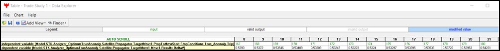
Table Page
Viewing the Data Explorer Toolbar
Once the trade study is complete and all data has been collected, the Data Explorer toolbar becomes active.
Data Explorer Tool Bar
Plotting the results
Some trade study tools will automatically launch a default plot window when the trade study runs. For other plots, you can create them from the Add View drop-down menu.
Viewing the data
There are multiple views that you can selecte to visualize the data seen on the Table Page. You can choose views by clicking Add View. You can build custom views or switch to Legacy Views.
- Close the 2D Scatter Plot that opened when you ran the trade study.
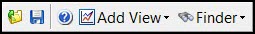
- On the Table Page tool bar, expand Add View.
- Select 2D Line Plot.
Setting axis variables
Use the Dimensions menu option to set which variable is displayed on which axis. In certain plots, you can also set other global plot controls based on the plot variables.
- Click Dimensions.
- Open the x drop-down menu and select Trip.
- Click the chart to close the Dimensions window.
- Slide your cursor to the bottom point in the chart.
The resulting plot shows the Delta-V required for each of the 21 runs. The true anomaly at which the least Delta-V is required occurs around 173 degrees.
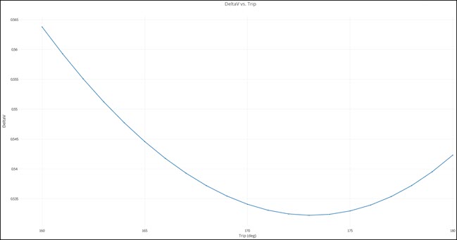
DeltaV vs Trip
Closing the tools
To get a more precise answer, you could rerun this analysis for values ranging from 172 degrees to 174 degrees.
- Close the Data Explorer window.
- When asked if you want to save, click .
- Close the Parametric Study.
Closing the Data Explorer window also closes the chart.
Using the Optimization Tool
The Optimization Tool is a collection of optimization algorithms that you can use within Analyzer. Many algorithms are available, including gradient based optimizers, genetic algorithms, multiobjective algorithms, and other heuristic search methods (see Algorithm Comparison Chart). A common graphical user interface is provided to define optimization problems. An algorithm selection wizard is also provided to make it easy to choose algorithms that will work best for the problem at hand.
The Parametric Study provides the ability to change one variable and examine the effect on another one. Further minimize the Delta-V required by varying the thrust direction in addition to true anomaly. In this instance, vary azimuth and elevation from - 25 degrees to +25 degrees.
- Return to Analyzer.
- In the STK Variables field, select Satellite ().
- In the STK Property Variables field, expand () the following in the order as shown:
- Propagator (Astrogator) ()
- TargetMnvr1 ()
- Mnvr1 ()
- Finite_ThrustVector ()
- Double-click Azimuth () to move it to the Analyzer Variables field..
- Double-click Elevation () to move it to the Analyzer Variables field.
- In the Analyzer tool bar select the Optimization Tool.

Optimization Tool Icon
Minimizing Delta-V
Once again, the objective is to minimize Delta-V.
- In the Component Tree, using your left mouse button, drag DeltaV () to the Objective field on the right.
- Ensure Goal is set to Minimize.
- In the Component Tree, using your left mouse button, drag Trip (), Azimuth () and Elevation () to the Design Variables field on the right.
- Make the following changes to the design value settings:
- Set Algorithm to Darwin.
- In the lower-right corner of the Optimization Tool, click .
- Close the 2D Scatter Plot.
| Option | Lower Bound | Upper Bound |
|---|---|---|
| Trip | 160 | 180 |
| Azimuth | -25 | 25 |
| Elevation | -25 | 25 |
Darwin is a genetic search algorithm developed specifically for solving constrained engineering optimization problems.
Analyzer Tool Bar Analyzer Icon
Be patient. This can take a few minutes.
The optimizer will display a history of steps as it progresses. By default only the objective definition will be displayed.
When the optimization study is complete, the Table page will contain the convergence history of the process. The last design point in the Table view will contain the optimized values. These values are also displayed in the Component Tree and the Value column for the design variables in the Optimization Tool.
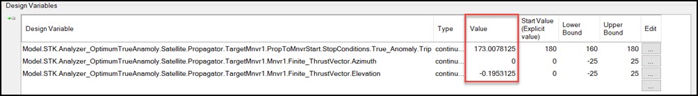
Design Variable Values
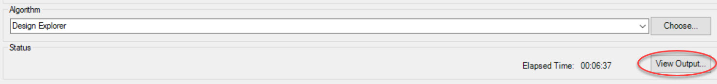
Viewing the Optimization Tool Output
You can view the Optimization Tool Output at any time and update during the optimization run using the Refresh button. The Optimization Tool Output dialog box has six tabs, each displaying different information about the optimization run. You can copy each page as an image and, if applicable, as text using the Copy button.
- Click .
- Select the Best Design tab.
- If desired, click each tab in the Optimization Tool Results window to get an idea of the information that is reported in each field.
- When finished, close the Optimization Tool Results window.
- Close the Design Explorer window.
- When asked if you want to save, click .
- Close the Optimization Tool.
- When the Optimization Tool query window appears, click .
- Close Analyzer.
If the problem formulation is single-objective, the Best Design tab appears, showing the last design improvement reported by the algorithm. By clicking , you can transfer the information in the report to a document or a slide show presentation.
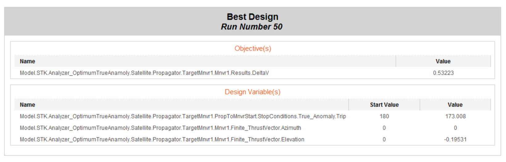
Best Design
These results are an example and might not match your results for data values and best design.
Using Analyzer and Astrogator, you were able to determine which true anomaly and other adjustments minimized Delta-V and saved fuel.
Save your work
- Save (
 ) your work.
 - Close your scenario.
Exercise Two: Launch error study
In this exercise, use Analyzer to determine what impact small launch errors can have on the mission. For this study, vary burnout latitude, longitude, altitude, and velocity and look at the resulting changes in Keplerian elements.
Using a starter scenario
To speed things up and have you to focus on the portion of this exercise that teaches you Analyzer, a partially created scenario has been provided for you.
Loading the starter scenario
The STK scenario (VDF) used with this tutorial is included with the STK installation. To open the scenario:
- Launch the STK® () application.
- Click Open a Scenario in the Welcome to STK dialog.
- Select Installed Scenarios in the navigation pane or browse to <STK install folder>\Data\ExampleScenarios.
Select the VDF
- Select Analyzer_LaunchErrors.vdf.
- Click .
Saving the starter scenario as an SC file
When you open the scenario, the STK application will create a folder with the same name as the scenario in the default user folder (C:\Users\<username>\Documents\STK_ODTK 13, for example). The STK application will not save the scenario automatically. When you choose save a scenario, the STK application will default to saving it in the format in which it originated. Therefore, if you open a VDF, the default save format will be a VDF. The same is true for a scenario file (*.sc). To save the VDF as an SC file, change the file format using the Save As procedure:
- Open the File menu.
- Select Save As....
- Select the STK User folder in the navigation pane when the Save As dialog box opens.
- Select the folder with the same name as the scenario.
- Click .
- Select Scenario Files (*.sc) in the Save as type drop-down list.
- Select the Scenario file in the file browser.
- Click .
- Click in the Confirm Save As Dialog box to overwrite the existing scenario file in the folder and to save your scenario.
A scenario folder with the same name as the VDF was created for you when you opened the VDF in the STK application. This folder contains the temporarily unpacked files from the VDF.
Viewing the satellite segments
Familiarize yourself with the orbital parameters of the satellite.
- Right-click Sat1 () in the Object Browser and select Properties ().
- On the Basic - Orbit page, go to the Mission Control Sequence (MCS).
Viewing the launch Segment: WallopsLaunch
The satellite starts with a Launch (![]() ) segment.
) segment.
- In the MCS, select WallopsLaunch (
 ).
). - Using the tabs at the top of the page, note the Launch and Burnout parameters.
Viewing the Propagate Segment: PropToAscendingNode
The satellite is moved to its ascending node using a Propagate (![]() ) segment.
) segment.
- In the MCS, select PropToAscendingNode (
 ).
). - Note the Stopping Condition.
Viewing the Target Sequence: RaiseApogee
The satellite's apoapsis (apogee) is raised using a Target (![]() ) sequence.
) sequence.
- In the MCS, select the Maneuver () segment named Mnvr1 ().
- X (Velocity) has been targeted (
 ).
). - Select the Propagate () segment named ToApogee (
 ). Note the stopping condition.
 - At the bottom of the MCS, click .
- In the Multi-Component Select Window, Altitude is the selected result.
- Close the Multi-Component Select Window.
Viewing the Differential Corrector
A Differential Corrector Profile runs the Target (![]() ) sequence.
) sequence.
- Select RaiseApogee ().
- Click the Profile Properties () icon.
- Close () the Targeting Profile window.
Looking at the Variables, the control parameter is Cartesian X (X (Velocity)), which was targeted. The equality constraint is altitude and the desired value of 2000 kilometers was set.
Viewing the Target Sequence: RaisePerigee
The satellite's periapsis (perigee) is raised using a Target (![]() ) sequence.
) sequence.
- Select the Maneuver () segment named Impulsive Maneuver ()
- At the bottom of the MCS, click .
- In the Multi-Component Select Window, Eccentricity and Inclination are the selected results.
- Close the Multi-Component Select Window.
Look at the Attitude Control. Both X(Velocity) and Y (Normal) have been targeted ().
Viewing the Differential Corrector
A Differential Corrector Profile runs the Target (![]() ) sequence.
) sequence.
- Select RaisePerigee ().
- Click the Profile Properties () icon.
- Close () the Targeting Profile window.
- Click to close Sat1's () properties.
Looking at the Variables, the control parameters are Cartesian X (X (Velocity)) and Cartesian Y (Y (Normal)) which were targeted. The equality constraints are eccentricity and inclination. The desired eccentricity value of 0 and inclination of 50 degrees were set.
Opening Analyzer
Click the Analyzer () button on the Analyzer Tool Bar.
Study the effect of variations of rocket burnout on the final orbital parameters. Vary burnout latitude, longitude, altitude, and fixed velocity and assess their impact on the six (6) Keplerian elements.
Setting the Input Variables
- In the STK Variables field, select Sat1 ().
- In the STK Property Variables field, expand () the following in the order as shown:
- Propagator (Astrogator) ()
- WallopsLaunch (
 )
) - Double-click the following variables to move them to the Analyzer Variables list:
- BurnoutVelocity_FixedVelocity ()
- Burnout_Geodetic_Latitude ()
- Burnout_Geodetic_Longitude ()
- Burnout_Geodetic_Altitude ()
Setting the Output Variables
- In the STK Property Variables field, expand () the following in the order as shown:
- Propagator (Astrogator) ()
- Prop10Mins ()
- FinalState ()
- Keplerian ()
- Double-click the following variables to move them to the Analyzer Variables list:
- SemiMajorAxis ()
- Eccentricity ()
- Inclination ()
- RAAN ()
- ArgOfPeriapsis ()
- TrueAnomaly ()
Using the Probabilistic Analysis Tool
The Probabilistic Analysis Tool helps you understand how uncertainties in the design parameters affect the outputs of the Analyzer model. The tool is typically used to compute the probability that the value of an output variable exceeds a specified limit. In addition to random sampling methods such as the Monte Carlo method, the tool provides a number of additional analytical methods that require much smaller sample sizes. You can set up and execute the probabilistic analysis through a unified graphical user interface (GUI). Using the GUI, you can easily switch between available algorithms.
In the Analyzer toolbar, click the Probabilistic ( ) icon.
Setting the Design Variables
- When the Probabilistic Analysis Tool opens, drag BurnoutVelocity_FixedVelocity () to the Design Variables list.
Selecting Distributions for Design Variables
It is important to properly specify the distribution characteristics of the design variables. When a new design variable is added to the tool, the Distribution Selection dialog box will appear.
Using the Distribution Selection dialog box, you can choose a distribution for a given design variable. It supports the following probabilistic distributions:
- Normal - This is a "bell-shaped" distribution that describes many situations where observations are distributed symmetrically around the mean. For this distribution, 68% of all values under the curve lie within one standard deviation of the mean, and 95% lie within two standard deviations.
- Uniform - This is a "flat" distribution in which all possible solutions between the lower bound and upper bound are equally likely.
- Lognormal - This is a probability distribution in which the log of the random variable follows the normal distribution. The log normal distribution is commonly used for general reliability analysis, fatigue failures, material strengths, and loading variables.
- Weibull - This is a distribution defined by shape and scale parameters. Two special cases of this distribution are: 1) the distribution is an exponential distribution when the shape parameter equals to 1, and 2) the distribution is a Rayleigh distribution when shape parameter equals to 2. This distribution is often used for modeling device failure rate and wind speeds.
- Triangle - This is a triangle-shaped distribution that is defined by a center point that is the mean and the population density slants off linearly to the lower bound and upper bound. You must specify all three parameters to completely define the distribution.
- Enumerated - This is a distribution with a list of discrete values, all of which are equally probable. The discrete values specified should be separated by commas.
- Deterministic - If a design variable value is to be fixed, use this distribution.
In this exercise, use the Normal distribution for all four (4) design variables.

Distribution Selection and Settings
- Leave the default Mean setting as is.
- Change the Std. Dev setting to 0.001% and then click .
- Drag Burnout_Geodetic_Latitude () to the Design Variables list.
- Change the Std. Dev setting to 0.001% and then click .
- Drag Burnout_Geodetic_Longitude () to the Design Variables list.
- Change the Std. Dev setting to 0.001% and then click .
- Drag Burnout_Geodetic_Altitude () to the Design Variables list.
- Change the Std. Dev setting to 0.001% and then click .
Running the study
- In the Components list, using your Shift key, select all six (6) Keplerian elements (SemiMajorAxis, Eccentricity, Inclination, RAAN, ArgOfPeriapsis, and TrueAnomaly) and drag them to the Responses field.
- Use the default Monte Carlo method.
- Change Number of Runs to 100.
- Click .
Monte Carlo is a random sampling technique. It generates random values for the design variables based on the joint distribution of the design variables. The samples are then evaluated for computing response variable values. Since this is a random sampling technique, if Analyzer performs a high enough number of evaluations, this method will give the most accurate results. The number of evaluations to generate a good probability estimate increases rapidly as the probability value under consideration decreases. Since Monte Carlo is a random sampling technique, you can use it with response functions, discrete design variables, and discrete response variables that are not smooth. The histogram plot ignores failed runs while calculating mean, variance, skewness, kurtosis, etc.
Plotting the Histogram
Use the Histogram page to visualize the distribution of a variable in a trade study. In addition to a graphical Histogram representation of the data, the page also contains a Box plot of the distribution as well as a display of the statistics of the distribution, including mean, standard deviation, quantiles, etc. Finally, the Histogram page contains bounds on which values of the variable are acceptable and computes reliability statistics based on how many runs fall into that defined space.
In this case, the Histogram Plot shows data for the first variable in the Responses field, SemiMajorAxis.
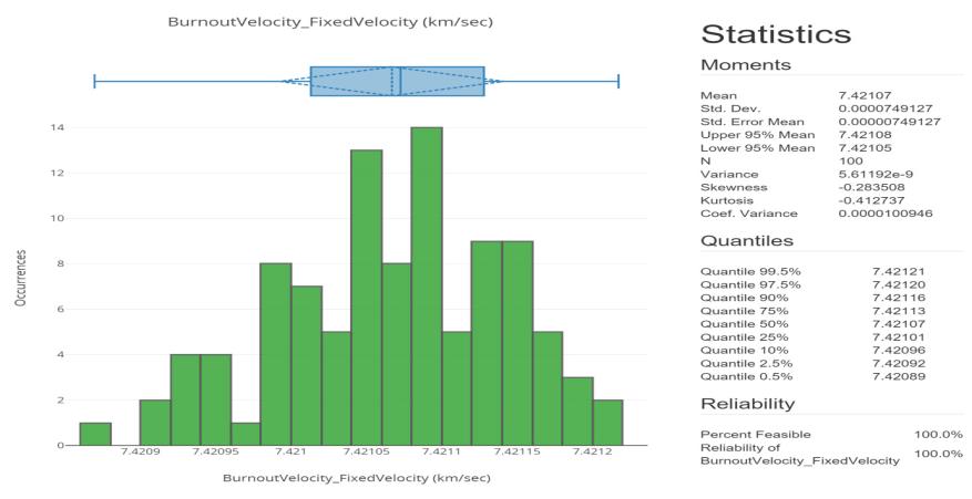
Histogram Plot
To view Histogram Plots on the remaining Keplerian Elements, do the following:
- In the upper-left corner of the plot, click Dimensions.
- Open the x drop-down menu and select Eccentricity.
- Click the plot to close the Dimensions window.
- You can cycle through each Keplerian Element in this manner.
Generating a scatter matrix
The Scatter Matrix displays a grid of graphs that compare every design variable and response against every other design variable and response in the trade study. Using these graphs, it's possible to quickly gain understanding as to the relationship between various variables in the trade study.
- Using the Histogram Plot toolbar, click Add View.
- Select Scatter matrix.
- When finished, close the Data Explorer windows.
- When prompted to save, click .
- Close the Probabilistic Analysis Tool.
- Close Analyzer.

Histogram Plot Toolbar

Scatter Matrix
Save your work
- Save () your work.
- Close your scenario.
Exercise 3: To the Moon
Now that you are more familiar with the interaction between Astrogator and Analyzer, analyze a more complex scenario. Once again you are trying to determine the Delta-V used, but this time you want to analyze the relationship between Delta-V and the time it takes to get from a low-Earth orbit into a low-altitude lunar orbit. Minimizing Delta-V is once again a concern, but you also want to keep the transfer time within an acceptable range.
Using a starter scenario
To speed things up and have you to focus on the portion of this exercise that teaches you Analyzer, a partially created scenario has been provided for you.
Loading the starter scenario
The STK scenario (VDF) used with this tutorial is included with the STK installation. To open the scenario:
- Launch the STK® () application.
- Click Open a Scenario in the Welcome to STK dialog.
- Select Installed Scenarios in the navigation pane or browse to <STK install folder>\Data\ExampleScenarios.
Select the VDF
- Select Analyzer_LunarMission.vdf.
- Click .
Saving the starter scenario as an SC file
When you open the scenario, the STK application will create a folder with the same name as the scenario in the default user folder (C:\Users\<username>\Documents\STK_ODTK 13, for example). The STK application will not save the scenario automatically. When you choose save a scenario, the STK application will default to saving it in the format in which it originated. Therefore, if you open a VDF, the default save format will be a VDF. The same is true for a scenario file (*.sc). To save the VDF as an SC file, change the file format using the Save As procedure:
- Open the File menu.
- Select Save As....
- Select the STK User folder in the navigation pane when the Save As dialog box opens.
- Select the folder with the same name as the scenario.
- Click .
- Select Scenario Files (*.sc) in the Save as type drop-down list.
- Select the Scenario file in the file browser.
- Click .
- Click in the Confirm Save As Dialog box to overwrite the existing scenario file in the folder and to save your scenario.
A scenario folder with the same name as the VDF was created for you when you opened the VDF in the STK application. This folder contains the temporarily unpacked files from the VDF.
Reviewing the Mission Control Sequence (MCS)
The Lunar Probe is launched into a Low Earth Orbit (LEO) transfer orbit and propagates until the trans-lunar injection burn. After the burn, it is further propagated until it reaches perilune, the point at which a spacecraft in lunar orbit is closest to the moon. At that time, another burn is performed to place the Lunar Probe into orbit around the Moon.
- Right-click LunarProbe () in the Object Browser and select Properties ().
- On the Basic - Orbit page, go to the Mission Control Sequence (MCS).
There are two targeting profiles for Target Moon. The first one gets the satellite close to the Moon and targets on Δ (delta) right ascension and Δ declination as well as the duration from translunar injection (TLI) burn until the satellite reaches the Moon.
Targeting the moon
- Select Target Moon.
- In the Profiles field, select Differential Corrector.
- Select Properties ().
- Close the Differential Corrector.
Note the Control Parameters and the desired Equality Constraints (Results).
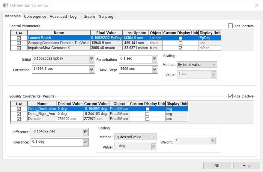
Target Moon
The second targeting profile targets the b-plane and gets the satellite into the desired lunar orbit.
- Select Differential Corrector1.
- Select Properties ().
Note the Control Parameters and the desired Equality Constraints (Results).
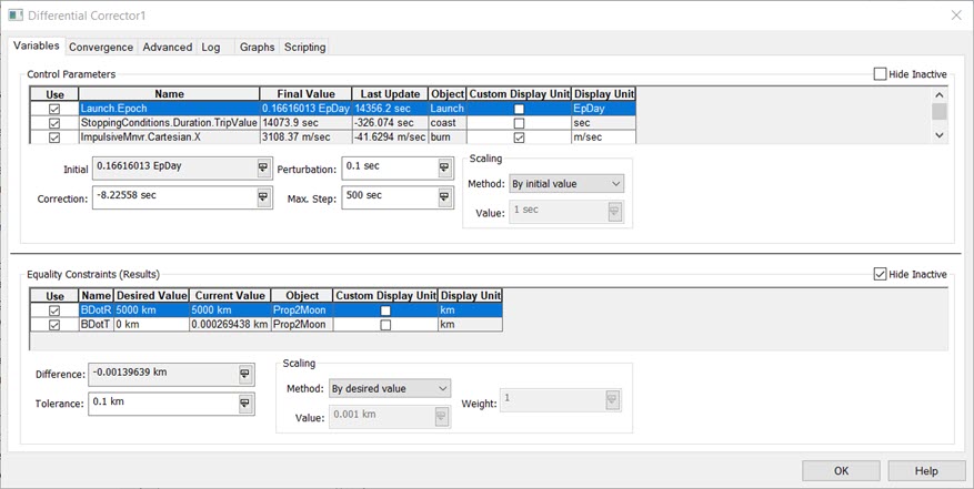
Establish Orbit
Changing the differential corrector
Make a change with this second differential corrector before moving on.
- Under Equality Constraints (Results), change the desired value of BDotR to 6000 km.
- Click .
- Click the Run Entire Mission Control Sequence (
 ) button.
 - Close the results windows.
Three windows will appear that inform you of the results of each differential corrector run. There is a differential corrector for Establish Lunar Orbit that places the Lunar Probe in a circular orbit.
Changing the time of flight
In this exercise, you want to change the time of flight and determine the required TLI Delta-V.
- Return to the MCS.
- Select burn (
 ).
). - Click at the bottom of the MCS.
- Expand (
 ) Maneuver.
 - Select DeltaV () and add () it to the results list.
- Click .
- Click to close LunarProbe's properties.
Opening Analyzer
Click the Analyzer () button on the Analyzer Tool Bar.
Setting the input variable
In the STK Variables field, select LunarProbe (![]() ).
).
- In the STK Property Variables field, expand () the following in the order as shown:
- Propagator (Astrogator) ()
- Target Moon ()
- Profiles ()
- Differential_Corrector ()
- EqualityConstraints ()
- Duration ()
- Double-click DesiredValue () to move it to the Analyzer Variables list.
Setting the output variable
- In the STK Property Variables field, expand () the following in the order as shown:
- Burn (
 )
) - Results ()
- Double-click DeltaV () to move it to the Analyzer Variables list.
Running Parametric Study
- In the Analyzer tool bar, select Parametric Study (
 ).
). - Set DesiredValue () as the Design Variable.
- Set the following design values:
- Set DeltaV () as the response.
- Click .
- Close the 2D Scatter Plot that opened when you ran the trade study.
- On the Table Page tool bar, expand Add View and select 2D Line Plot.
| Option | Value |
|---|---|
| starting value | 200000 |
| ending value | 500000 |
| number of samples | 7 |
| step size | 50000 |
The omputations can take a couple of minutes, so stick with a small number of steps for now. The values are in seconds.
Changing the Dimensions
- Click Dimensions.
- Open x drop-down menu and select DesiredValue.
- Click the chart to close the Dimensions window.
Checking the results
Based on the chart, Design Point: 4, 350000 seconds (approximately 4.1 days) returns the lowest DeltaV.

Parametric Study
On your own
The required thrust varies slightly during the month. Using Analyzer’s Carpet Plot Study Tool, vary the starting time by 30 days (one data point/day) and analyze the amount of Delta-V required to reach the Moon when launching on different days.
- When finished, close any reports you have open and the Data Explorer window.
- When prompted to save, click .
- Close the any Analysis Tools you are using.
- Close Analyzer.
Save your work
- Save () your work.
- Close your scenario.