STK Premium (Air), STK Premium (Space), or STK Enterprise
You can obtain the necessary licenses for this tutorial by contacting AGI Support at support@agi.com or 1-800-924-7244.
Required product install: A 64-bit version of Java is required to run Analyzer. See the Analyzer system requirements for more information.
The results of the tutorial may vary depending on the user settings and data enabled (online operations, terrain server, dynamic Earth data, etc.). It is acceptable to have different results.
Capabilities covered
This lesson covers the following capabilities:
- STK Pro
- STK Analyzer
- Coverage
- Communications
Analyzer
Analyzer is integrated into the STK workflow to help you automate and analyze STK trade studies in order to better understand the design of your system. For purposes of this tutorial, you will use Analyzer to:
- Perform Trade Studies. Analyzer will enable you to quickly perform “what if” studies so that you can understand how changing various scenario parameters will impact the scenario.
- Optimize Scenario Parameters. Once you understand the key parameters of a scenario, you will use an optimizer to drive the scenario to an optimal configuration.
Setting tutorial activities
In this tutorial, you will do the following:
- Analyze a STK Communications Scenario for trends.
- Optimize Communications Scenario parameters to meet mission objectives.
This tutorial is designed to teach you how to explore the STK design space in order to optimize your communications scenario. You will learn how to perform Parametric, Carpet Plot, and Optimization studies that vary input variables through a range of values, resulting in plots of one or more output variables.
Defining the tutorial
The goal of this scenario is to analyze a satellite in geosynchronous orbit (GEO) that will communicate with facilities spanning the contiguous United States (CONUS). Think of the coverage grid points as being locations of communication sites. The Coverage Definition object enables you to use a custom point file, which would come in handy should you have actual locations of your communication sites. You need to better understand the requirements for the GEO satellite transmitter. In particular this includes specifying communications parameters for the transmitter. This study will focus on the ratio of energy per bit to noise spectral density (Eb/No).
To better understand how the GEO satellite transmitter parameters impact coverage capabilities, you will run a series of parametric studies. For each parametric study, you will run a single design parameter through a sweep of values. At each value, you'll collect coverage statistics using a Figure of Merit object.
Your goal for this problem is to optimally configure the satellite’s transmitter to best provide link closure to all facilities via a high Eb/No. There are a handful of parameters that will impact your study:
- Power
- Frequency
- Data Rate
- antenna dish size
To initiate the analysis, perform a few parametric studies to see how changing each of these parameters impacts the coverage capability. You'll follow this by creation of a carpet plot to view how multiple parameters impact coverage. Lastly, you'll do an optimization study to scan through the design space to find a solution that meets requirements.
Video Guidance
Watch the following video. Then follow the steps below, which incorporate the systems and missions you work on (sample inputs provided).Please note, the video refers to a starter scenario accessed from the STK Data Federate (SDF). This scenario is included with your STK install. Please follow the written steps in this tutorial to open the file.
Using a starter scenario
To speed things up and have you to focus on the portion of this exercise that teaches you Analyzer, a partially created scenario has been provided for you.
Loading the starter scenario
The STK scenario (VDF) used with this tutorial is included with the STK installation. To open the scenario:
- Launch the STK® (
 ) application.
 - Click
 Open a Scenario in the Welcome to STK dialog.
 - Select Installed Scenarios in the navigation pane or browse to <STK install folder>\Data\ExampleScenarios.
Opening the VDF
- Select Analyzer_Comm_Analysis.vdf.
- Click .
Saving the starter scenario as an SC file
When you open the scenario, the STK application will create a folder with the same name as the scenario in the default user folder (C:\Users\<username>\Documents\STK_ODTK 13, for example). The STK application will not save the scenario automatically. When you choose save a scenario, the STK application will default to saving it in the format in which it originated. Therefore, if you open a VDF, the default save format will be a VDF. The same is true for a scenario file (*.sc). To save the VDF as an SC file, change the file format using the Save As procedure:
- Open the File menu.
- Select Save As....
- Select the STK User folder in the navigation pane when the Save As dialog box opens.
- Select the folder with the same name as the scenario.
- Click .
- Select Scenario Files (*.sc) in the Save as type drop-down list.
- Select the Scenario file in the file browser.
- Click .
- Click in the Confirm Save As Dialog box to overwrite the existing scenario file in the folder and to save your scenario.
A scenario folder with the same name as the VDF was created for you when you opened the VDF in the STK application. This folder contains the temporarily unpacked files from the VDF.

2D Graphics Window
Determining Eb/No
In the 2D Graphics window, Geo_Sat’s antenna is boresighted at the geographic center of the contiguous United States (Centroid). The color contours represent the Eb/No dB of the transmission.
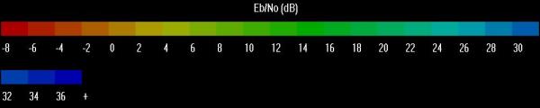
Eb/No Legend
- In the Object Browser, right-click EbNo_Avg (
 ) and select the Report & Graph Manager (
 ).
). - In the Installed Styles list, select the Grid Stats report and click .
- Close the report and the Report & Graph Manager.
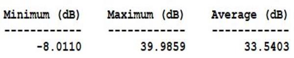
Grid Stats Report
The contours are based on the minimum and maximum values in the report.
Noting the Analyzer layout
Use the Analyzer Main Form to configure input/output variables available for further analysis. You can first select an object in the scenario tree on the left. When you select an object, Analyzer lists all possible input variable candidates under the Inputs General tab and the Inputs Constraints tab. It lists all output variable candidates under the Outputs Data Providers tab, Outputs Object Coverage tab, Outputs DeckAccess tab, or Outputs MissileModelingTools tab.
Determining the impacts of power on coverage
The first study you will perform varies power to determine which value is best. You need to select input and output variables from the main Analyzer window to pass to the Parametric Study tool.
Select the input variable.
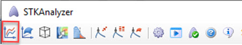
- Click the Analyzer button on the Analyzer Tool Bar.
- In the STK Variables list, expand Geo_Sat and then expand Tgt_Centroid.
- Select DL_Tx.
- In the STK Property Variables field, expand Model (Complex_Transmitter_Model) and then ModelSpecs.
- Double-click Power. This moves Power to the Analyzer Variables field as an input.
Analyzer Tool Bar Analyzer Icon
Another way of opening Analyzer is to go to the Object Browser, right-click the scenario object (or any object), select the object's Plugins, and click Analyzer.
Selecting the output variables.
- In the Object Browser, expand CONUS_Cov and select EbNo_Avg.
- In the Data Provider Variables field, expand Overall Value and double-click the following items to move them into the Analyzer Variables field:
- Minimum
- Maximum
- Average
Using the Parametric Study Tool
The Parametric Study Tool runs a scenario through a sweep of values for some input variable. You can plot he resulting data to view trends.
- In the Analyzer tool bar, select Parametric Study.
- When the Parametric Study opens, in the Component Tree, using your left mouse button, drag Power to the Design Variable field on the right.
- Set the following Design Variables:
- In the Component Tree, using your left mouse button, drag Minimum, Maximum, and Average to the Responses field on the right.
- In the lower-right corner of the Parametric Study Tool, click .
Parametric Study Icon
Analyzer builds a parametric representation of the currently loaded scenario. This representation appears in the Component Tree displayed on the left side of each trade study tool.
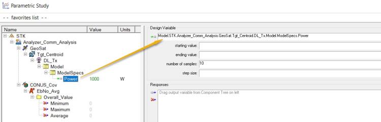
Design Variable
| Option | Value |
|---|---|
| starting value | 300 |
| ending value | 3000 |
| number of samples | 10 |
| step size | 300 |
Using Data Explorer
Data Explorer is a tool used by Trade Study tools to display data while they are being collected from STK. While data are being collected, the Data Explorer displays a progress meter, a halt button, and the data.
Viewing the Table page
The Table page displays trade study data in a tabular form. It is the default window that is present for all trade studies. Cells are shaded differently depending on the associated variable's state. Input variables are shown with green text, valid values are displayed with black text, invalid values are displayed with gray text, and modified values are displayed with blue text. From the table it is possible to view and edit all values in your trade study and even to add and remove whole runs.
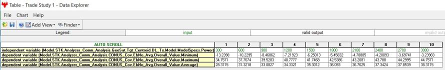
Table Page
Viewing the Toolbar
Once the trade study is complete and all data has been collected, the Data Explorer toolbar becomes active.

Data Explorer Tool Bar
Generating plots
Some trade study tools will automatically launch a default plot window when the trade study runs. For other plots, you can create them from the Add View drop-down menu.
Selecting views
There are multiple views that you can select to visualize the data seen on the Table page. You can choose views by clicking on Add View.
- Close the 2D Scatter Plot that opened when you ran the trade study.
- On the Table Page tool bar, expand Add View.
- Select the 2D Line plot.
Setting plot axes
Use the Dimensions menu option to set which variable is displayed on which axis. In certain plots, you can set other global plot controls based on the plot variables.
- Click Dimensions.
- Open the x drop-down menu and select Power.
- In the Dimensions tool bar and select the plus (+) button.
- Change Series 2 (x) to Power and change (y) to Maximum. This adds Maximum to the plot.
- In the Dimensions tool bar and select the plus (+) button.
- Change Series 3 (x) to Power and change (y) to Average. This adds Average to the plot.
- Click the plot to close the Dimension menu.
The chart now shows Minimum vs Power. Obviously, you could change y to Maximum or Average plots. However, you will add Maximum and Average to the plots results for comparison on one plot.
Set options for the axes
Use the Axes tab to set options for the axes.
- Click Axes.
- Select the Ticks tab.
- Change the Max # value to 40.
- Click the plot to close the Axes menu.
- Close the 2D Line Plot and the Table Page.
- When prompted to save, select .
- Return to the Parametric Study Tool.

Custom 2D Line Plot
Rerunning with adjusted values
Adjust the Power Design Variable values by a factor of 10.
- Increase Power Design Variables by setting the following values:
- Click .
- Close the 2D Scatter Plot that opened when you ran the trade study.
- On the Table Page tool bar, expand Add View .
- Select the 2D Line plot.
- Close the 2D Line Plot and the Table Page.
- When prompted to save, select .
- Close the Parametric Study Tool.
- Return to Analyzer.
| Option | Value |
|---|---|
| starting value | 3000 |
| ending value | 30000 |
| number of samples | 10 |
| step size | 3000 |
This study gives you an understanding of which power setting to use for the transmitter to give the best overall minimum Eb/No. This tutorial is focusing on Power vs Minimum at 0 dB. Looking at the 2D Line plot, you can see that this is reached with a power level somewhere between 6000 and 9000 watts. You could continue to refine the Parametric Study until you find the desired value. Furthermore, you could enter that value in the Parametric Study Tool's component list under Power Value which is editable and sync that value back to STK.
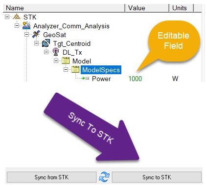
Edit and Sync to STK
Determining the impacts of frequency on coverage
Power is not the only transmitter parameter that will impact your coverage. Frequency also has an impact. To determine how much, run another Parametric Study.
Select the input variable.
- In the STK Variables list, expand Geo_Sat and then expand Tgt_Centroid.
- Select DL_Tx.
- In the STK Property Variables field, expand Model (Complex_Transmitter_Model) and then ModelSpecs.
- Double-click Frequency. This moves Frequency to the Analyzer Variables field as an input.
- In the Analyzer tool bar, select Parametric Study.
- In the Component Tree, using your left mouse button, drag Frequency to the Design Variable field on the right.
- Set the following Design Variables:
- In the Component Tree, using your left mouse button, drag Minimum, Maximum, and Average to the Responses field on the right.
- In the lower right hand corner of the Parametric Study Tool, click .
- Close the 2D Scatter Plot that opened when you ran the trade study.
- On the Table Page tool bar, expand Add View.
- Select the 2D Line plot.
| Option | Value |
|---|---|
| starting value | 10 |
| ending value | 20 |
| number of samples | 11 |
| step size | 1 |
Setting the axes
- Click Dimensions.
- Open the x drop-down menu and select Frequency.
- In the Dimensions tool bar and select the plus (+) button.
- Change Series 2 (x) to Frequency and change (y) to Maximum. This adds Maximum to the plot.
- In the Dimensions tool bar and select the plus (+) button.
- Change Series 3 (x) to Frequency and change (y) to Average. This adds Average to the plot.
- Click the plot to close the Dimension menu.
- Close the 2D Line plot and the Table Page.
- When prompted to save, select .
- Close the Parametric Study Tool.
- Return to Analyzer.
The chart now shows Minimum vs Frequency. Obviously, you could change y to Maximum or Average plots. However, you will add Maximum and Average to the plots results for comparison on one plot.
This study gives you an understanding of what frequency band to use for the transmitter which provides the best overall minimum Eb/No. Eb/No decreases with frequency due to an increase in propagation loss and decrease in Gaussian Antenna gain, where Gaussian is the default antenna type you are using on the transmitter. You can see that frequencies < 13 GHz will assure you of an Eb/No > 0 for all of CONUS.
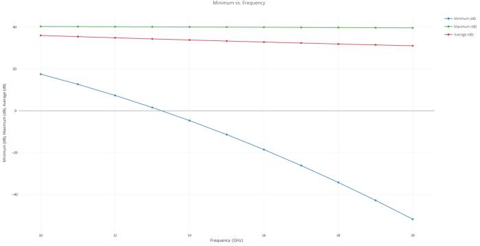
Custom 2D Line Plot
Determining the impacts of data rate on coverage
The next parameter impacting coverage is the data rate of the transmitter. For this study, you will vary the data rate from 10 to 20 Mb/sec (megabits per second).
Select the input variable.
- In the STK Variables list, expand Geo_Sat and then expand Tgt_Centroid.
- Select DL_Tx.
- In the STK Property Variables field, expand Modulator.
- Double-click DataRate. This moves DataRate to the Analyzer Variables field as an input.
- In the Analyzer tool bar select Parametric Study.
- In the Component Tree, using your left mouse button, drag DataRate to the Design Variable field on the right.
- Set the following Design Variables:
- In the Component Tree, using your left mouse button, drag Minimum, Maximum and Average to the Responses field on the right.
- In the lower right hand corner of the Parametric Study Tool, click .
- Close the 2D Scatter Plot that opened when you ran the trade study.
- On the Table Page tool bar, expand Add View and select the 2D Line plot.
| Option | Value |
|---|---|
| starting value | 10e+06 |
| ending value | 20e+06 |
| number of samples | 11 |
| step size | 1e+06 |
Setting the plot axes
- Click Dimensions.
- Open the x drop-down menu and select DataRate.
- In the Dimensions tool bar and select the plus (+) button.
- Change Series 2 (x) to DataRate and change (y) to Maximum. This adds Maximum to the plot.
- In the Dimensions tool bar and select the plus (+) button.
- Change Series 3 (x) to DataRate and change (y) to Average. This adds Average to the plot.
- Click the plot to close the Dimension menu.
The chart now shows Minimum vs DataRate. Obviously, you could change y to Maximum or Average plots. However, you will add Maximum and Average to the plots results for comparison on one plot.

Data Rate Change
Coverage decreases with increased data rate. Decreasing the data rate equivalently decreases the bandwidth and increases the Eb/No.
- Close the 2D Line Plot and the Table Page.
- When prompted to save, select .
- Close the Parametric Study Tool.
- Return to Analyzer.
Determine the impacts of antenna size on coverage
The next parameter you will examine is the size of the antenna dish for the transmitter. Although this isn't part of the transmitter's optimization, it's an interesting study. For this study, vary the dish size from 0.5 to 2 m (meters).
Select the input variable.
- In the STK Variables list, expand Geo_Sat and then expand Tgt_Centroid.
- Select DL_Tx.
- In the STK Property Variables field, expand Antenna and then ModelSpec.
- Double-click Diameter. This moves Diameter to the Analyzer Variables field as an input.
- In the Analyzer tool bar select Parametric Study.
- In the Component Tree, using your left mouse button, drag Diameter to the Design Variable field on the right.
- Set the following Design Variables:
- In the Component Tree, using your left mouse button, drag Minimum, Maximum, and Average to the Responses field on the right.
- In the lower-right corner of the Parametric Study Tool, click .
- Close the 2D Scatter Plot that opened when you ran the trade study.
- On the Table Page tool bar, expand Add View and select the 2D Line plot.
| Option | Value |
|---|---|
| starting value | 0.5 |
| ending value | 2 |
| number of samples | 16 |
| step size | 0.1 |
Setting the plot axes
- Click Dimensions.
- Open the x drop-down menu and select Diameter.
- In the Dimensions tool bar and select the plus (+) button.
- Change Series 2 (x) to Diameter and change (y) to Maximum. This adds Maximum to the plot.
- In the Dimensions tool bar and select the plus (+) button.
- Change Series 3 (x) to Diameter and change (y) to Average. This adds Average to the plot.
- Click the plot to close the Dimension menu.
- Close the 2D Line Plot.
The chart now shows Minimum vs Diameter. Obviously, you could change y to Maximum or Average plots. However, you will add Maximum and Average to the plots results for comparison on one plot.
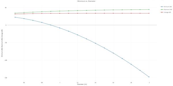
Antenna Size Change
Notice that while the maximum and for the most part average Eb/No values rise with increasing antenna size, the minimum value decreases. The maximum coverage value increases with increasing antenna diameter, however you do see diminishing returns. The reason for this is that as antenna size increases, the gain increases while the Beamwidth decreases. Locations farthest from the antenna boresight see their Eb/No values drop as the Beamwidth decreases. Take a closer look at the average coverage.
Looking closer at the average
- On the Table page, expand Add View and select 2D Line Plot.
- Expand Dimensions and make the following changes:
- Select Axes.
- Select the Ticks tab and change Max # to 20.
- Click the 2D Line Plot.
- Close the 2D Line Plot and the Table Page.
- When prompted to save, click .
- Close the Parametric Study Tool.
- Return to Analyzer.
| Option | Value |
|---|---|
| x | Diameter |
| y | Average |
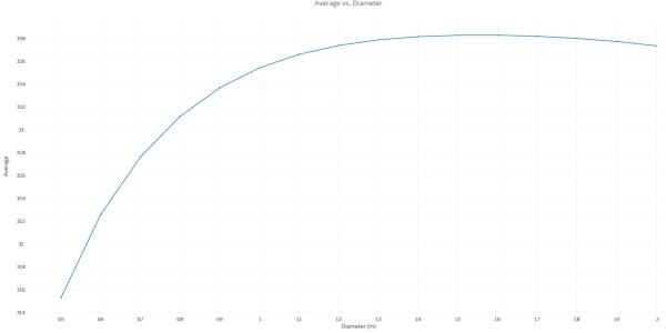
Eb/No vs Antenna Size (Average)
The average Eb/No value reaches a peak value at an antenna diameter of about 1.5 m (meters) and then the average Eb/No values begin to decrease.
Determining if power and frequency impact one another
You have determined that power and frequency have significant impacts on coverage capability while data rate has less of an influence. Power has an increasingly positive impact. Frequency has a negative influence. This leads to the following question:
How do frequency and power affect one another?
You can answer the question by performing a two-dimensional parametric study called a Carpet Plot.
Using the Carpet Plot Tool
A Carpet Plot is a means of displaying data dependent on two variables in a format that makes interpretation easier than normal multiple curve plots. A Carpet Plot can be thought of as a multidimensional Parametric Study.
- In the Analyzer tool bar, select Carpet Plot.
- In the Component Tree, using your left mouse button, drag Frequency to the first Design Variable field on the right and Power to the second Design Variable field.
- Set the following Frequency Design Variables:
- Set the following Power Design Variables:
- In the Component Tree, using your left mouse button, drag Minimum to the Responses field on the right.
- In the lower-right corner of the Carpet Plot Tool, click .
- Close the Carpet Plot and the Table Page.
- When prompted to save, select .
- Close the Carpet Plot Tool.
- Return to Analyzer.

Carpet Plot Icon
Setting the design variables is similar to using the Parametric Study Tool except you now have two variables instead of one.
| Option | Value |
|---|---|
| From | 10 |
| To | 20 |
| Num Steps | 5 |
| Step Size | 2.5 |
| Option | Value |
|---|---|
| From | 3000 |
| To | 30000 |
| Num Steps | 6 |
| Step Size | 5000 |
If you are wondering why this tutorial uses large step sizes, it's due to keeping the tutorial time under an hour. These settings will require a total of thirty runs to obtain every variable combination. On your own, you can set the frequencies and power to change at smaller step sizes to make the trade study more realistic. Be patient. Depending on your settings, you could end up executing hundreds of runs.
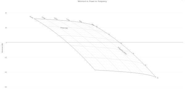
Carpet Plot
Using the Carpet Plot you can determine combinations of frequency and power desired for your requirement which is an Eb/No of 0 dB.
Optimizing transmitter parameters
You now know that transmitter parameters have a large impact on coverage capabilities. To optimize these parameters, you can either guess at values, or employ an optimization tool. Although you can clearly see trends from the previous studies, guessing at values will be difficult because you are dealing with multiple parameters at the same time and the trends you have studied thus far assume only one or two parameters are changed at a time.
To solve more complex problems, an optimization tool can be a very useful guide. An optimizer is an automated tool that makes mathematical calculations about a design problem and incrementally attempts to find an optimal solution. The algorithm you will employ here is an optimizer. The selected algorithm will compute derivatives about an initial point in the design space and compute a search direction. This process will repeat until no more progress can be achieved on the objective function.
You will use an optimizer in this problem to minimize the power requirement for the transmitter while maintaining a minimum coverage capability of 0 dB for the coverage area.
Using the Optimization Tool
The Optimization Tool is a collection of optimization algorithms that you can use within Analyzer. Many algorithms are available, including gradient-based optimizers, genetic algorithms, multiobjective algorithms, and other heuristic search methods (see Algorithm Comparison Chart). A common graphical user interface is provided to define optimization problems. An algorithm selection wizard is also provided to make it easy to choose algorithms that will work best for the problem at hand.
- In the Analyzer tool bar, select the Optimization Tool.
- In the Component Tree, using your left mouse button, drag Power to the Objective field on the right.
- Ensure the Goal field is set to Minimize.
- In the Component Tree, using your left mouse button, drag Minimum to the Constraint field on the right.
- Set the Lower Bound to 0 (zero) and the upper bound to 10 (ten).
- In the Component Tree, using your left mouse button, drag Power, Frequency, and DataRate to the Variable field on the right.
- Make the following changes:
- Set Algorithm to Darwin.
- In the lower-right corner of the Optimization Tool, click .
- Close the 2D Scatter Plot.
Optimization Tool Icon
The objective is to minimize the value for power by changing frequency, data rate, and power all while maintaining a minimum Eb/No value of as close to 0 to 10 dB as possible.
| Option | Lower Bound | Upper Bound |
|---|---|---|
| Power | 300 | 30000 |
| Frequency | 10 | 20 |
| DataRate | 10e6 | 20e6 |
Darwin is a genetic search algorithm developed specifically for solving constrained engineering optimization problems.
The optimizer will display a history of steps as it progresses. By default, it will display only the objective definition.
You can repeat the above process to add plots for frequency and data rate.
Viewing the results
When the optimization study is complete, you can view the convergence history of the process and see the best design.
- Click on the Optimization Tool panel to reveal the convergence history of the process.
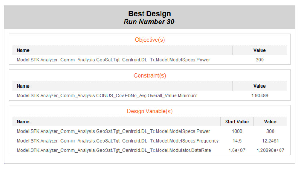
- Select the Best Design tab, which will contain the optimized values. These values are also displayed in the Value column for the design variables in the Optimization Tool. See the images below.
- Click to push these parameters to the scenario.
- Recompute the Coverage analysis
- Right-click CONUS_Cov.
- Extend the CoverageDefinition menu.
- Select Compute Access.
- Regenerate the Grid Stats Report
- In the Installed Styles list, select the Grid Stats report and click .
- In the Object Browser, right-click EbNo_Avg () and select the Report & Graph Manager ().
This result was generated with a different algorithm and so is just an example. Your resulting data and best design may be different.

Optimization Parameters
The optimizer was able to drive power to its lower bound of 300 W while at the same time attaining the goal of between 0 and 10 dB of minimum Eeb/Nn for all time.
If you create a final Grid Stats Report you obtain the following:
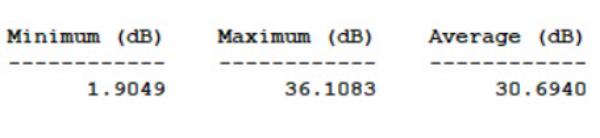
Final Grid Stats Report
You can compare your 2D Graphics view with the original legend:
You can enable the legend on the Figure of Merit - 2D Graphics - Static page.

Final 2D Graphics Window View
When you finish
- Close the Table Page, the Optimization Tool, Analyzer, the Report & Graph Manager, and any open reports.
- Save your work.
- Close the scenario.
- Close STK.