Analyzer: Performing Communications Interference Trade Studies
STK Premium (Air), STK Premium (Space), or STK Enterprise
You can obtain the necessary licenses for this tutorial by contacting AGI Support at support@agi.com or 1-800-924-7244.
Required product install: A 64-bit version of Java is required to run Analyzer. See the Analyzer system requirements for more information.
The results of the tutorial may vary depending on the user settings and data enabled (online operations, terrain server, dynamic Earth data, etc.). It is acceptable to have different results.
Capabilities Covered
This lesson covers the following capabilities:
- STK Pro
- STK Analyzer
- Coverage
- Communications
Analyzer
STK's Analyzer capability is integrated into the STK workflow to help you automate and analyze STK trade studies in order to better understand the design of your system. For purposes of this tutorial, Analyzer will be used to:
- Parametrically explore the STK design space in order to analyze your Communications Interference Scenario.
- Perform parameter studies that vary an input variable through a range of values and plot one or more output variables.
Video Guidance
Watch the following video. Then follow the steps below, which incorporate the systems and missions you work on (sample inputs provided).
Please note, the video refers to a starter scenario accessed from the STK Data Federate (SDF). This scenario is included with your STK install. Please follow the written steps in this tutorial to open the file.
Satellite Communications Interference Exercise
A satellite (GeoSat) in geosynchronous orbit is being used to communicate with various communication sites throughout the contiguous United States (CONUS). Think of the coverage grid points as being locations of communication sites. The Coverage Definition object allows you to use a custom point file which would come in handy should you have actual locations of your communication sites. A satellite in a low Earth orbit (Leo_Sat) is interfering with these communications.
To better understand how LeoSat's transmitter parameters impact coverage, a series of parametric studies will be run. For each parametric study, a single design parameter will be run through a sweep of values. At each value, coverage statistics will be collected using a Figure of Merit.
The goal for this problem is to study LeoSat’s transmitter settings to evaluate how EIRP (Equivalent Isotropically Radiated Power) and frequency affect minimum energy per bit to noise power spectral density ratio plus interference Eb/(No+Io) across the coverage grid.
To initiate the analysis, perform a few parameter studies to see how changing each of these parameters impacts the coverage. This will be followed by creation of a carpet plot to view how multiple parameters impact coverage.
Using a starter scenario
To speed things up and have you to focus on the portion of this exercise that teaches you Analyzer, a partially created scenario has been provided for you.
Loading the starter scenario
The STK scenario (VDF) used with this tutorial is included with the STK installation. To open the scenario:
- Launch the STK® (
 ) application.
 - Click
 Open a Scenario in the Welcome to STK dialog.
 - Select Installed Scenarios in the navigation pane or browse to <STK install folder>\Data\ExampleScenarios.
Opening the VDF
- Select Analyzer_Interference_Analysis.vdf.
- Click .
Saving the starter scenario as an SC file
When you open the scenario, the STK application will create a folder with the same name as the scenario in the default user folder (C:\Users\<username>\Documents\STK_ODTK 13, for example). The STK application will not save the scenario automatically. When you choose save a scenario, the STK application will default to saving it in the format in which it originated. Therefore, if you open a VDF, the default save format will be a VDF. The same is true for a scenario file (*.sc). To save the VDF as an SC file, change the file format using the Save As procedure:
- Open the File menu.
- Select Save As....
- Select the STK User folder in the navigation pane when the Save As dialog box opens.
- Select the folder with the same name as the scenario.
- Click .
- Select Scenario Files (*.sc) in the Save as type drop-down list.
- Select the Scenario file in the file browser.
- Click .
- Click in the Confirm Save As Dialog box to overwrite the existing scenario file in the folder and to save your scenario.
A scenario folder with the same name as the VDF was created for you when you opened the VDF in the STK application. This folder contains the temporarily unpacked files from the VDF.

2D Graphics Window
Scenario Overview
Geo_Sat’s antenna, Geo_Tx, is boresighted at the geographic center of the contiguous United States (Centroid). Geo_Tx, was optimally configured to provide a minimum energy per bit to noise power spectral density ratio (Eb/No) of ~ 0 dB anywhere within CONUS. Geo_Tx's settings are:
- Frequency: 12.5551 GHz
- Power: 300 watts (24.7712 dBW)
- Data Rate: 12.4693 Mb/sec
Leo_Sat's transmitter, Leo_Tx, is transmitting with the following settings:
- Frequency: 12.5551 GHz
- EIRP: 1000 watts (30 dBW)
Interference
Leo_Tx is transmitting on the same frequency as Geo_Tx.
The CommSystem object, CommSystem1, has been configured to determine if Leo_Tx is interfering with the communications between Geo_Tx and DL_Rx (Centroid's receiver). DL_Rx is being used as CONUS_Cov's constraint object on the grid definition inside of CONUS. The Coverage Figure of Merit Object, EbNo_Io, was set up to determine if interference is occurring on the grid points throughout CONUS. Based on this set up, you will run two reports. The first report will determine if Leo_Tx is interfering with DL_Rx. The second report will determine how Leo_Tx is affecting the grid points throughout CONUS.
Receiver Interference
How is Leo_Tx affecting DL_RX?
- In the Object Browser, right-click on CommSystem1 and select the Report & Graph Manager.
- In the Installed Styles list, select Link Information Detailed.
- Click .
- Scroll to the right of the report and locate the Eb/No (dB) and Eb/(No+Io) (dB) columns. The Eb/No (dB) column shows the communications without interference and the Eb/(No+Io) (dB) shows if there is interference.
- Scroll down through the report until you locate areas where the Eb/(No+Io) (dB) shows interference on the communications link. The below report is a sample with the Time, Eb/No, and Eb/(No+Io).
- Close the report and the Report & Graph Manager.
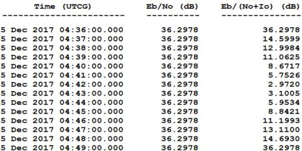
Eb/No Interference Sample
You can see from the report, that there is occasional interference against DL_Rx.
Coverage Interference
How is Leo_Tx affecting the coverage grid?
- In the Object Browser, right-click on EbNo_Io and select the Report & Graph Manager.
- Generate a Grid Stats Over Time report.
- Scroll down the report until you see evidence of interference.
- Bring the 2D Graphics window to the front.
- Start the scenario.
- When finished, Reset the scenario.
- Close the report and the Report & Graph Manager.
The Minimum (dB) values are mostly 0 dB. However, when Leo_Tx is interfering with the coverage grid, you will see those values dipping below 0 dB.
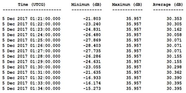
Grid Interference Sample
You will see more grid interference due to each point in the CONUS grid being evaluated instead of Centroid's receiver. The contours on the 2D and 3D Graphic windows are set for the minimum to cut off at -1 dB.
Remember, the original goal was to always have an Eb/No of ~ 0 dB throughout CONUS. Whenever Leo_Tx is dropping the Eb/No below -1 dB in the coverage grid, contour color will disappear.
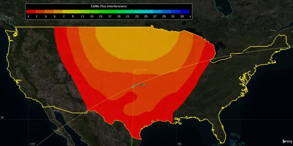
2D Graphics Grid Interference Sample
Analyzer Layout
Use the Analyzer Main Form to configure input/output variables available for further analysis. You can first select an object in the scenario tree on the left. When an object is selected, all possible input variable candidates are listed under the Inputs General tab and the Inputs Constraints tab. All output variable candidates are listed under the Outputs Data Providers tab, Outputs Object Coverage tab, Outputs DeckAccess tab or Outputs MissileModelingTools tab.
Determine the Impacts of EIRP on Coverage
The first study you will perform varies EIRP to determine which value produces the greatest interference. You need to select input and output variables from the main Analyzer window to pass to the Parametric Study tool.
Select the input variable.
- Click the Analyzer button on the Analyzer Tool Bar.
- When Analyzer is open, in the STK Variables list, expand Leo_Sat.
- Select Leo_Tx.
- In the STK Property Variables field, expand Model (Simple_Transmitter_Model) and then ModelSpecs.
- Double-click EIRP. This moves EIRP to the Analyzer Variables field as an input.
- In the Variables list, expand CONUS_Cov and select EbNo_Io.
- In the Data Provider Variables field, expand Overall Value and double-click the following fields to move them into the Analyzer Variables field as outputs:
- Minimum
- Maximum
- Average
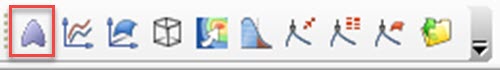
Analyzer Tool Bar Analyzer Icon
Another way of opening Analyzer is to go to the Object Browser, right click on the scenario object (or any object), select the object's Plugins, and click Analyzer.
Parametric Study Tool
The Parametric Study Tool runs a Scenario through a sweep of values for some input variable. The resulting data can be plotted to view trends.
- In the Analyzer tool bar select Parametric Study.
- When the Parametric Study opens, in the Component Tree, using your left mouse button, drag EIRP to the Design Variable field on the right.
- Set the following Design Variables:
- In the Component Tree, using your left mouse button, drag Minimum, Maximum, and Average to the Responses field on the right.
- In the lower right hand corner of the Parametric Study Tool, click .
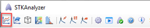
Parametric Study Icon
Analyzer builds a parametric representation of the currently loaded Scenario. This representation is viewed in the Component Tree displayed on the left side of each trade study tool.
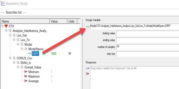
Design Variable
| Option | Value |
|---|---|
| starting value: | 100 |
| ending value: | 10100 |
| number of samples: | 11 |
| step size: | 1000 |
Data Explorer
The Data Explorer is a tool used by Trade Study tools to display data while they are being collected from STK. While data is being collected, the Data Explorer displays a progress meter, a halt button, and the data.
Table Page
The Table page displays trade study data in a tabular form. It is the default window that is present for all trade studies. Cells are shaded differently depending on the associated variable's state. Input variables are shown with green text, valid values are displayed with black text, invalid values are displayed with gray text, and modified values are displayed with blue text. From the table it is possible to view and edit all values in your trade study and even to add and remove whole runs.
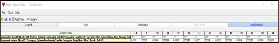
Table Page
The Figure of Merit object (EbNo_Io) was configured with the following settings:
- Across Assets: Maximum (Constraint values are computed for all currently available assets and the maximum is selected.)
- Compute: Minimum (The minimum value of the samples of the dynamic definition of the access constraint.)
The results of your trade studies will show maximum minimum values throughout.
Toolbar
Once the trade study is complete and all data has been collected, the Data Explorer toolbar becomes active.

Data Explorer Toolbar
Plot Types
Some trade study tools will automatically launch a default plot window when the trade study runs. Other plots can be created from the Add View dropdown menu.
Views
There are multiple views that can be selected to visualize the data seen on the Table Page. You can choose views by clicking on Add View. You can build custom views or switch to Legacy Views. You will try both. Start with a legacy view which will allow you to quickly view all three results on the same plot.
- Close the 2D Scatter Plot that opened when you ran the trade study.
- On the Table Page tool bar, expand Add View and select 2D Line plot.
Dimensions
Use the Dimensions menu option to set which variable is displayed on which axis. In certain plots, you can set other global plot controls based on the plot variables.
- Click Dimensions.
- Open x pull down menu and select EIRP.
- In the Dimensions tool bar and select the plus (+) button.
- Change Series 2 (x) to EIRP and change (y) to Maximum. This adds Maximum to the plot.
- In the Dimensions tool bar and select the plus (+) button.
- Change Series 3 (x) to EIRP and change (y) to Average. This adds Average to the plot.
- Click on the plot to close the Dimension menu.
The chart now shows Minimum vs EIRP. Obviously, you could change y to Maximum or Average plots. However, you will add Maximum and Average to the plots results for comparison on one plot.
Axes
Use the Axes tab to set options for the axes.
- Click Axes.
- Select the Ticks tab.
- Change the Max # value to 20.
- Click on the plot to close the Axes menu.
- Close the 2D Line Plot and the Table Page.
- When prompted to save, select .
- Return to the Parametric Study Tool.
- Close the Parametric Study Tool.
- Return to Analyzer.
The plot is similar to the Legacy 2D Line Plot. There are other edits you can make if desired.
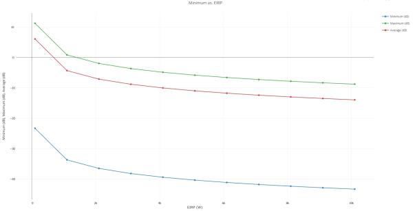
2D Line Plot
Determine the Impacts of Frequency on Coverage
EIRP is not the only transmitter parameter that will impact your coverage. Frequency also has an impact. To determine how much, run another Parametric Study.
Select the input variable.
- In the STK Variables list, expand Leo_Sat.
- Select Leo_Tx.
- In the STK Property Variables field, expand Model (Simple_Transmitter_Model) and then ModelSpecs.
- Double-click Frequency. This moves Frequency to the Analyzer Variables field as an input.
- In the Analyzer tool bar select Parametric Study.
- In the Component Tree, using your left mouse button, drag Frequency to the Design Variable field on the right.
- Set the following Design Variables:
- In the Component Tree, using your left mouse button, drag Minimum, Maximum, and Average to the Responses field on the right.
- In the lower right hand corner of the Parametric Study Tool, click .
- Close the 2D Scatter Plot that opened when you ran the trade study.
| Option | Value |
|---|---|
| starting value: | 12.5 |
| ending value: | 12.6 |
| number of samples: | 11 |
| step size: | 0.01 |
Generating the 2D Line Plot
- On the Table Page tool bar, expand Add View and select the 2D Line plot.
- Click Dimensions.
- Open x pull down menu and select Frequency.
- In the Dimensions tool bar and select the plus (+) button.
- Change Series 2 (x) to Frequency and change (y) to Maximum. This adds Maximum to the plot.
- In the Dimensions tool bar and select the plus (+) button.
- Change Series 3 (x) to Frequency and change (y) to Average. This adds Average to the plot.
- Click on the plot to close the Dimension menu.
- Close the 2D Line Plot and the Table Page.
- When prompted to save, select .
- Close the Parametric Study Tool.
- Return to Analyzer.
The chart now shows Minimum vs Frequency. Obviously, you could change y to Maximum or Average plots. However, you will add Maximum and Average to the plots results for comparison on one plot.

Frequency Change
This study gives you an understanding of what frequency band creates the lowest overall minimum Eb/(No+Io). Eb/(No+Io) decreases with frequency as the frequency of the interferer approaches the frequency of the desired transmitter. We can see that frequencies < 12.52 GHz and > 12.59 GHz will assure us of an Eb/(No+Io) ~ 0dB for all of CONUS.
Determine if EIRP and Frequency Impact One Another
You have determined that EIRP and frequency have significant impacts on coverage. This leads to the following question:
How do frequency and power affect one another?
You can answer the question by performing a 2-dimensional parametric study called a Carpet Plot.
Carpet Plot Tool
A Carpet Plot is a means of displaying data dependent on two variables in a format that makes interpretation easier than normal multiple curve plots. A Carpet Plot can be thought of as a multi-dimensional Parametric Study.
- In the Analyzer tool bar select Carpet Plot.
- In the Component Tree, using your left mouse button, drag Frequency to the first Design Variable field on the right and EIRP to the second Design Variable field.
- Set the following Frequency Design Variables:
- Set the following EIRP Design Variables:
- In the Component Tree, using your left mouse button, drag Minimum to the Responses field on the right.
- In the lower right hand corner of the Carpet Plot Tool, click .

Carpet Plot Icon
Setting the design variables is similar to using the Parametric Study Tool except you now have two variables instead of one.
| Option | Value |
|---|---|
| From | 12.5 |
| To | 12.6 |
| Num Steps | 3 |
| Step Size | 0.05 |
| Option | Value |
|---|---|
| From | 100 |
| To | 1000 |
| Num Steps | 3 |
| Step Size | 500 |
If you are wondering why this tutorial uses large step sizes, it's due to keeping the tutorial time under an hour. These settings will require a total of nine runs to obtain every variable combination. On your own, you can set the frequencies and EIRP to change at smaller step sizes to make the trade study more realistic. Be patient. Depending on your settings, you could end up running hundreds of runs.

Carpet Plot
Using the Carpet Plot, basing the study on an Eb/No of 0 dB, you can determine combinations of frequency and EIRP that creates the most interference in the coverage grid.
When You Finish
- Close the Carpet Plot, Table Page, the Carpet Plot tool, Analyzer, the Report & Graph Manager, and any open reports.
- Save your work.
- Close the scenario.
- Close STK.