STK Pro, STK Premium (Air), STK Premium (Space), or STK Enterprise
You can obtain the necessary licenses for this tutorial by contacting AGI Support at support@agi.com or 1-800-924-7244.
This lesson requires STK 12.9 or newer to complete in its entirety. If you have an earlier version of STK, you can complete a legacy version of this lesson.
The results of the tutorial may vary depending on the user settings and data enabled (online operations, terrain server, dynamic Earth data, etc.). It is acceptable to have different results.
Capabilities covered
This lesson covers the following STK Capabilities:
- STK Pro
Problem statement
You are using STK for preliminary analysis of a future air traffic control radar system that will track aircraft flying through an airport's control zone. You are also interested in determining if a low earth orbit (LEO) satellite can take pictures of a ground site in the training area.
Solution
Use STK to model a scenario that allows you to consider and compare all of your system options. Simulate an aircraft traveling in the vicinity of the airport and use a
Video guidance
Watch the following video. Then follow the steps below, which incorporate the systems and missions you work on (sample inputs provided).
Creating a scenario
Start by creating a scenario.
- Click
 Create a Scenario in the Welcome to STK dialog box.
 - Enter the following in the New Scenario Wizard:
- Click when finished.
- Click Save (
 ) when the scenario loads. A folder with the same name as your scenario is created for you in the location specified above.
 - Verify the scenario name and location.
- Click .
| Option | Value |
|---|---|
| Name | SensorIntro |
| Location: | Default |
| Start | 1 Jul 2016 16:00:00.000 UTCG |
| End | + 1 day |
Turning off Terrain Server
If you plan to complete the L3 quiz at the end of the tutorial, turn off the Terrain Server.![]()
Save Often!
Creating the Airport Radar Site
Start by creating the radar site.
- Insert a Place (
 ) object using the Insert Default method.
 - Rename the Place object RadarSite.
- Open RadarSite's () properties (
 ).
). - Select the Basic - Definition page.
- Make the following changes:
- Click .
| Option | Value |
|---|---|
| Latitude | 38.8006 deg |
| Longitude | -104.6784 deg |
| Height Above Ground: | 50 ft |
The additional 50 feet of altitude above the ground is to simulate the height of the radar antenna.
Viewing the Radar Site
View the Radar Site (![]() ) in the 3D Graphics Window.
) in the 3D Graphics Window.
- Right click on RadarSite () in the Object Browser.
- Select Zoom To.
- Bring the 3D Graphics window to the front.
- Use your left and right mouse buttons to obtain situational awareness of where your radar site is located.
Creating waypoints
The test aircraft will fly between two waypoints. For the test, you will insert two additional Place objects using the City Database.
Inserting a Place object located at Cheyenne, Wyoming
- Insert a Place () object using the From City Database method (
 ).
). - Type Cheyenne in the Name: field in the Search Standard Object Data dialog box.
- Click .
- Select Cheyenne, Wyoming in the Results: list.
- Click .
Inserting a Place object located at Raton, New Mexico
- Return to the Search Standard Object Database dialog box.
- Type Raton in the Name: field.
- Click .
- Select Raton, New Mexico in the Results: list.
- Click .
- Click to close the Search Standard Object Data dialog box.
Viewing the places
View the three Place (![]() ) objects in the 2D Graphics Window.
) objects in the 2D Graphics Window.
- Bring the 2D Graphics window to the front.
- Locate your Place objects on the 2D Graphics window.
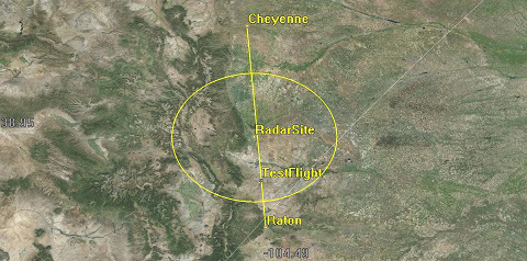
- Zoom in until you are centered on RadarSite with Cheyenne and Raton visible at the top and bottom of your map.
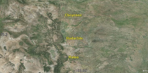
Place Object Locations
Inserting an aircraft
Insert an aircraft into your scenario.
- Insert an Aircraft (
 ) object using the Insert Default method.
 - Rename the Aircraft object "TestFlight".
Setting the aircraft Propagator
The aircraft performing the test flight will fly from Raton to Cheyenne. Since this is a preliminary analysis of the radar system, you can use the Great Arc Propagator.
- Open TestFlight's () properties ().
- Select the Basic - Route page.
- Note the Propagator is set to GreatArc.
Modeling the Test Flight Aircraft
You can also use the mouse to enter waypoints directly in the 2D Graphics window. Simply click anywhere in the 2D Graphics window to add new waypoints (latitude/longitude values) in the waypoint table. However, you must use the Route page to enter altitude, speed, and turn radius values. When you use the mouse to define a great arc route, it is recommended that you specify the altitude and speed for the first point before you create the second point, so that the initial route information become the default for all additional points.
If you plan to complete the L3 quiz at the end of the tutorial, follow these steps.![]()
Animating the test flight
Animate the test flight and view it in the 2D Graphics Window.
- Return to the 2D Graphics window.
- Make sure you can see the entire flight route of TestFlight.
- Use the Decrease Time Step (
 ) button in the Animation toolbar to decrease the time step to 3.00 sec.
 - Click the Start (
 ) button.
 - Observe your aircraft as it flies from Raton to Cheyenne.
- Click the Reset (
 ) button when finished.
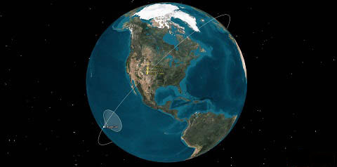
Modeling a LEO Satellite
Add a Satellite object to the scenario. You need to analyze when the satellite's camera (Sensor object) can take pictures of Raton.
- Insert a Satellite (
 ) object using the Orbit Wizard (
 ) method.
 - Make the following changes to the Orbit Wizard:
- Click .
| Option | Value |
|---|---|
| Type | Circular |
| Satellite Name | ImageSat |
| Inclination | 60 deg |
| Altitude | 800 km |
| RAAN | 20 deg |
Inserting a fixed sensor on a moving object
Use Sensor objects to model the various components that make up the detection system. Insert a default Sensor (![]() ) object. The default Sensor Object that STK creates when you introduce a Sensor object is a simple conic sensor with a 45 degree cone angle. The default view is fixed at zero (0) degrees azimuth and 90 degrees elevation which is nadir pointing. When a Sensor object is attached to a moving object it points with respect to the parent object’s reference frame. A fixed sensor is always pointing in a fixed direction with respect to its parent object.
) object. The default Sensor Object that STK creates when you introduce a Sensor object is a simple conic sensor with a 45 degree cone angle. The default view is fixed at zero (0) degrees azimuth and 90 degrees elevation which is nadir pointing. When a Sensor object is attached to a moving object it points with respect to the parent object’s reference frame. A fixed sensor is always pointing in a fixed direction with respect to its parent object.
- Insert a Sensor (
 ) object using the Insert Default method.
 - Select ImageSat () in the Select Object window.
- Click .
- Rename the Sensor1 () to Fixed.
Viewing the fixed sensor
View the sensor (![]() ) in the 3D Graphics window.
) in the 3D Graphics window.
- Bring the 3D Graphics window to the front.
- Right click on ImageSat () in the Object Browser.
- Select select Zoom To.
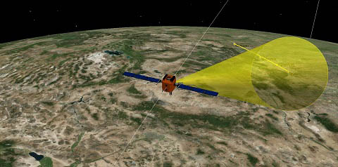
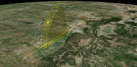
- Use your left and right mouse buttons to get a good view of ImageSat and the Sensor object's field of view and the locations of your ground sites.
Fixed Sensor
Calculating Access from Fixed sensor
The first analysis to perform is to check, whether or not, if Fixed will see Raton (![]() ) during your analysis period (24 hours).
) during your analysis period (24 hours).
- Right click on Fixed () in the Object Browser.
- Select Access... (
 ).
). - Select Raton () in the Associated Objects list in the Access Tool ().
- Click . in the Reports panel.
- Take a look at the report. During the 24 hour exercise, Raton will be in Fixed's field of view (FOV) a couple of times.
- Note the Total Duration time in the report.
- Close the report.
- Close the Access Tool.
Modeling a moving sensor on a moving object
When you attached the Fixed (![]() ) sensor, you used the default fixed pointing type. Many satellites can gimbal their sensors to track other objects (stationary and moving). STK provides a variety of Sensor object definitions and pointing types that allow you to model this type of movement.
) sensor, you used the default fixed pointing type. Many satellites can gimbal their sensors to track other objects (stationary and moving). STK provides a variety of Sensor object definitions and pointing types that allow you to model this type of movement.
Inserting the Targeted sensor on the satellite
First you will insert a sensor (![]() ) object called Targeted on ImageSat (
) object called Targeted on ImageSat (![]() ).
).
- Insert a Sensor () object using the Insert Default method.
- Select ImageSat () in the Select Object window.
- Click .
- Rename the Sensor1 () to Targeted.
Modeling the moving sensor
Update the sensor definition and pointing type to model the targeted sensor.
- Open Targeted's () properties ().
- Select the Basic - Definition page.
- Ensure the Sensor Type is set to Simple Conic.
- Change the Cone Half Angle: to 5 deg.
- Select the Basic - Pointing page.
- Change Pointing Type: to Targeted.
- Move (
 ) Raton () from the Available Targets list to the Assigned Targets list.
 - Click .
Calculating Access from Targeted sensor
Compare the access time between Targeted (![]() ) and Fixed (
) and Fixed (![]() ).
).
- Right click on Targeted () in the Object Browser.
- Select Access... ().
- Select Raton () in the Associated Objects list.
- Click in the Reports panel.
- Note the Total Duration time.
- Right-click on the first Access Start Time in the Access report.
- Select Start Time in the shortcut menu.
- Select Set Animation Time.
How does the access time for Targeted compare to Fixed? When you target the Sensor object, it locks onto the assigned target using the Sensor objects boresight. It's a point-to-point access. You're using the line-of-site constraint. Therefore, Targeted accesses Raton from horizon to horizon. The field of view for Fixed had to pass over Raton. So, the access time for Targeted is much higher.
Viewing Access in the 3D Graphics Window
- Bring the 3D Graphics window to the front.
- Zoom To ImageSat () if required to reset your view.
- Use your left and right mouse buttons to get a good view of ImageSat and the Sensor object's field of view and the locations of your ground sites.
- Click the Start () button on the Animation Toolbar to view any accesses that occur.
- Click the Reset () button when finished.
Targeted Access
Cleaning up your scenario
- Close the report.
- Close the Access Tool.
- Extend the Analysis menu.
- Select Remove All Accesses.
- Disable Fixed () in the Object Browser.
- Disable Targeted () in the Object Browser.
Your preliminary analysis shows that both cameras attached to ImageSat will have opportunities to take pictures of Raton.
Modeling the fixed sensor on a stationary object
You are now ready to model the radar field of view for RadarSite (![]() ). In the previous examples, you attached sensors to moving objects to model a fixed camera field of view and a camera that can gimbal. Sensors can also be used to model instruments attached to stationary objects, such as Facility, Place and Target objects. Fixed Sensor objects attached to stationary objects also point with respect to the parent object’s reference frame. Since stationary objects never change position or direction, a fixed Sensor object will always point in a fixed direction with respect to the parent object.
). In the previous examples, you attached sensors to moving objects to model a fixed camera field of view and a camera that can gimbal. Sensors can also be used to model instruments attached to stationary objects, such as Facility, Place and Target objects. Fixed Sensor objects attached to stationary objects also point with respect to the parent object’s reference frame. Since stationary objects never change position or direction, a fixed Sensor object will always point in a fixed direction with respect to the parent object.
Inserting the Radar Dome sensor on the Radar Site
First you will insert a sensor (![]() ) object called RadarDome on RadarSite (
) object called RadarDome on RadarSite (![]() ).
).
- Insert a Sensor () object using the Insert Default method.
- Select RadarSite () in the Select Object window.
- Click .
- Rename the Sensor3 () to RadarDome.
Updating the sensor's field-of-view
The Sensor object created here is similar to the fixed Sensor object attached to ImageSat (![]() ). However, it has a larger field-of-view. Change the Cone Half Angle to 90 deg.
). However, it has a larger field-of-view. Change the Cone Half Angle to 90 deg.
- Open RadarDome's () properties ().
- Select the Basic - Definition page.
- Change the Cone Half Angle to 90 deg.
- Click .
Adding constraints
RadarDome (![]() ) points straight up from RadarSite (
) points straight up from RadarSite (![]() ). It has an up looking field-of-view that covers everything above RadarSite (
). It has an up looking field-of-view that covers everything above RadarSite (![]() ). That’s not very realistic. Let’s limit its range so that the field-of-view spans a constrained area mimicking the field-of-view of the actual air traffic control radar.
). That’s not very realistic. Let’s limit its range so that the field-of-view spans a constrained area mimicking the field-of-view of the actual air traffic control radar.
- Select the Constraints - Active page.
- Click Add new constraints (
 ) in the Active Constraints toolbar.
 - Select Range in the Constraint Name list in the Select Constraints to Add dialog box.
- Click .
- Click to close the Select Constraints to Add dialog box.
- Select Max: in the Range panel of the Constraint Properties section.
- Enter 150 km in the Max: field.
- Click .
Viewing RadarDome in the 3D Graphics Window
View RadarDome (![]() ) in the 3D Graphics Window.
) in the 3D Graphics Window.
- Bring the 3D Graphics window to the front.
- Zoom To RadarSite ().
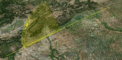
- Using your mouse, zoom out far enough so that you can see RadarDome's () full field-of-view.
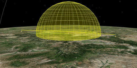
Radar Dome Field-of-View
Setting 2D Projection properties
2D Graphics Projection properties for Sensor objects control the display of sensor projection graphics in the 2D Graphics window. Sensor objects attached to Facility, Place and Target objects differ in their display behavior from those attached to vehicles. The intersections of Sensor objects with the Earth are displayed during animation. The Extension Distances option indicates whether the Sensor object’s field-of-view crossings at specified distances are computed and displayed in the 2D Graphics window. When the Sensor object display is set to project to the range constraint, STK projects the Sensor object's field-of-view to the maximum range specified on the Basic Constraints properties page for the Facility, Place, or Target object.
- Bring the 2D Graphics window to the front.
- Locate your Place objects and zoom in until you are centered on RadarSite with Cheyenne and Raton visible at the top and bottom of your map. At this point, there is no indication of RadarDome's field-of-view.
- Return to RadarDome's () properties ().
- Select the 2D Graphics - Projection page.
- Select Use Range Constraint as the Project to: option.
- Click .
- Return to the 2D Graphics window.
- You can see the range constraint of 150 km projecting out from RadarDome.
2D Graphics Projection
Calculating RadarDome's Access
There's no doubt visually, that RadarDome can access TestFlight. For the purposes of the analysis, we need to know for how long.
- Right click on RadarDome () in the Object Browser.
- Select Access... ().
- Select TestFlight () in the Associated Objects list.
- Click in the Reports panel.
- Click Report Units (
 ) at the top of the access report.
 - Ensure Time Dimension is selected on the left.
- Select Minutes (min) in the New Unit list.
- Click .
This is pretty straight forward. The access report tells you when and for how long you have access to TestFlight. For briefing purposes, you might want to change the duration from seconds to minutes.
Saving as Quick Report
Sometimes it's useful to change report units. You can save the report inside or outside of STK. Later, you will be sending this scenario to someone who does not have STK. Therefore, you can create a Quick Report. If you make any property changes to the objects being used in the access calculation, the changes will appear in the Quick Report. Therefore, if you want to compare numbers, sometimes it's a good idea to save reports externally. For the purposes of this scenario, there's no need. Should you decide to do this, you can use the Save as .csv icon.
- Click Save as quick report (
 ) at the top of the access report.
 - Close (
 ) the report.
 - Click the Quick Report Manager (
 ) at the top of STK.
 - Select the Access Quick Report.
- Click .
- Return to the Quick Report Manager.
- Click .
All of your Quick Reports will be available by simply opening the Quick Report Manager. You can rename your reports, add descriptions, delete them, etc.
Zooming to Access start time
You can use the report to quickly jump to the time in the scenario when RadarDome first accesses TestFlight.
- Return to the Access report.
- Right-click on the first Access Start Time in the Access report.
- Select Start Time in the shortcut menu.
- Select Set Animation Time.
- Bring the 3D Graphics window to the front.
- Zoom To TestFlight ().
- Using your mouse, move your view around so you can see TestFlight ()enter RadarDome ().
Generating an AER Report
This gives you a good idea of the location of TestFlight when it first enters RadarDome's field-of-view. You'll recall, that the maximum distance constraint for RadarDome is 150 km. Also, an air traffic controller might need to know TestFlight's azimuth and elevation data.
- Return to the Access Tool.
- Make sure RadarDome is selected as the Access For: object.
- Make sure TestFlight () is selected in the Associated Objects list.
- Click in the Reports panel.
- Scroll through the report. This report not only tells you what time RadarDome accesses TestFlight, but it reports the azimuth, elevation, and range.
Cleaning up your scenario
- Close the report.
- Close the Access Tool.
- Extend the Analysis menu.
- Select Remove All Accesses.
- Disable RadarDome () in the Object Browser.
Modeling a moving sensor on a stationary object
Often, the dome created by a Sensor object is used to model a field-of-view, or the overall volume of space in which radar looks. The radar itself often sweeps or scans through that field-of-view in a repeating cycle. The area of space represented by such a scanning or spinning radar at any given instant is its field-of-view. Add another level of fidelity to your scenario and build a sweeping radar beam using a moving Sensor object.
Inserting the Radar Sweep sensor on the Radar Site
First you will insert a sensor (![]() ) object called RadarSweep on RadarSite (
) object called RadarSweep on RadarSite (![]() ).
).
- Insert a Sensor () object using the Insert Default method.
- Select RadarSite () in the Select Object window.
- Click .
- Rename the Sensor3 () to RadarSweep.
Defining the Sensor's definition
You want to simulate the actual field-of-view, antenna height, and spinning properties of your air traffic control radar. The antenna height was set when you increased RadarSite's (![]() ) altitude earlier in the scenario.
) altitude earlier in the scenario.
Often, the area created by a sensor’s projection is used to model a field-of-view. Rectangular sensor types are typically used for modeling the field-of-view of instruments such as push broom sensors and star trackers. Rectangular sensors are defined according to specified vertical and horizontal half-angles.
The radar that you are modeling sweeps or scans in a repeating cycle. Since the radar “scans”, the full range of the radar is not always covered. You can configure the sensor’s field-of-view to provide a visual representation of the area that the radar does cover at any given point in time.
- Open RadarSweep's () properties ().
- Select the Basic - Definition page.
- Make the following changes:
| Option | Value |
|---|---|
| Sensor Type | Rectangular |
| Vertical Half Angle | 5 deg |
| Horizontal Half Angle | 35 deg |
The above configuration should create a wedge type field-of-view. Right now, that “wedge” is just pointing straight up.
Setting the Pointing Properties
Set the properties of the Sensor object to rotate and point at 35 degrees elevation. Set the RadarSweep's (![]() ) Pointing Type to Spinning. You can set the spin axis elevation to 90 degrees for horizontal rotation with a cone angle of 55 degrees for a 35 degree elevation from the horizon.
) Pointing Type to Spinning. You can set the spin axis elevation to 90 degrees for horizontal rotation with a cone angle of 55 degrees for a 35 degree elevation from the horizon.
- Return to RadarSweep's () properties ().
- Select the Basic - Pointing page.
- Make the following changes:
- Click .
| Option | Value |
|---|---|
| Pointing Type | Spinning |
| Spin Rate (Revs/Min) | 12 revs/min |
| Spin Axis - Cone Angle | 55 deg |
Setting the Constraints of the Sensor
Right now, the field-of-view extends beyond the limits of the actual radar because you haven’t constrained it. The airport’s primary surveillance radar has a range of 150 km. You need to limit the range of the radar to model that constraint.
- Select the Constraints - Active page.
- Click Add new constraints () in the Active Constraints toolbar.
- Select Range in the Constraint Name list in the Select Constraints to Add dialog box.
- Click .
- Click to close the Select Constraints to Add dialog box.
- Select Max: in the Range panel of the Constraint Properties section.
- Enter 150 km in the Max: field.
- Click .
Viewing the Radar Sweep sensor
View the RadarSweep (![]() ) sensor in the 3D Graphics window.
) sensor in the 3D Graphics window.
- Bring the 3D Graphics window to the front.
- Zoom to RadarSite ().
- Use your mouse and mouse buttons to get a good view the RadarSweep's () field-of-view.
- In order to view the RadarSweep () in real time, click the X Real-time Animation Mode icon in the Animation toolbar.
- Click the Start () to play the scenario. You can see RadarSweep as it turns 12 revolutions a minute.
- Reset () the scenario when finished.
Rectangular Sensor
Visualizing RadarSweep on the 2D Graphics Window
- Bring the 2D Graphics window to the front.
- Locate your Place objects and zoom in until you are centered on RadarSite with Cheyenne and Raton visible at the top and bottom of your map. At this point, there is no indication of RadarSweep's field-of-view.
- Return to RadarSweep's () properties ().
- Select the 2D Graphics - Projection page.
- Select Use Range Constraint as the Project to: option.
- Click .
- Return to the 2D Graphics window.
- Click the Start () button on the Animation Toolbar.
- Notice the sensor projection moving on the 2D Graphics Window.
- Click the Reset () button when finished.
Generating an access graph
Determine when RadarSweep (![]() ) has access to TestFlight (
) has access to TestFlight (![]() ) using an access graph.
) using an access graph.
- Right click on RadarSweep () in the Object Browser.
- Select Access... ().
- Select TestFlight () in the Associated Objects list.
- Click in the Graphs panel.
- Hold down the left mouse button and hover over an item on the graph.
- Draw a box around the item and zoom closer.
- Close () the access graph.
This graph is interesting because it's graphing each instance RadarSweep accesses TestFlight while it is spinning. The Zoom In tool is embedded in the functionality of the mouse.
Generating an access report
Generate an access report. You will then jump to an access time, so you can create a stored view at that time.
- Return to the Access Tool ().
- Click in the Reports panel.
- Right-click on the first Access Start Time.
- Select Start Time in the shortcut menu.
- Select Set Animation Time.
- Close () the Access report.
Creating a Stored Views
At times, you may desire to quickly return to a particular 3D Graphics view. For instance, you might use this scenario for a briefing. During the briefing, you desire to jump to the 3D Graphics window view of when TestFlight is first detected by RadarSweep. Store a view that depicts just that.
- Bring the 3D Graphics window to the front.
- Zoom To RadarSite ().
- Mouse around until you are happy with the view.
- Click Stored Views (
 ) on the 3D Graphics window toolbar.
 - Click .
- Rename View0 First Access.
- Click .
- Click Reset () in the Animation toolbar.
- Click Home View (
 ) in the 3D Graphics window toolbar.
 - Select First Access in the Stored Views pull down menu.
First Access
Calculating multiple Accesses
You can quickly create an access graph that shows all the Sensor objects at the same time. You can create the graph from TestFlight to the Sensor objects. The Sensor properties will still be used.
- Return to the Access Tool ().
- Click the .
- Select TestFlight in the Select Object dialog box.
- Click .
- Using your Ctrl key and mouse, select all four Sensor objects in the Associated Objects list. You may need to expand ImageSat or RadarSite to see all the Sensor objects.
- Click in the Graphs panel.
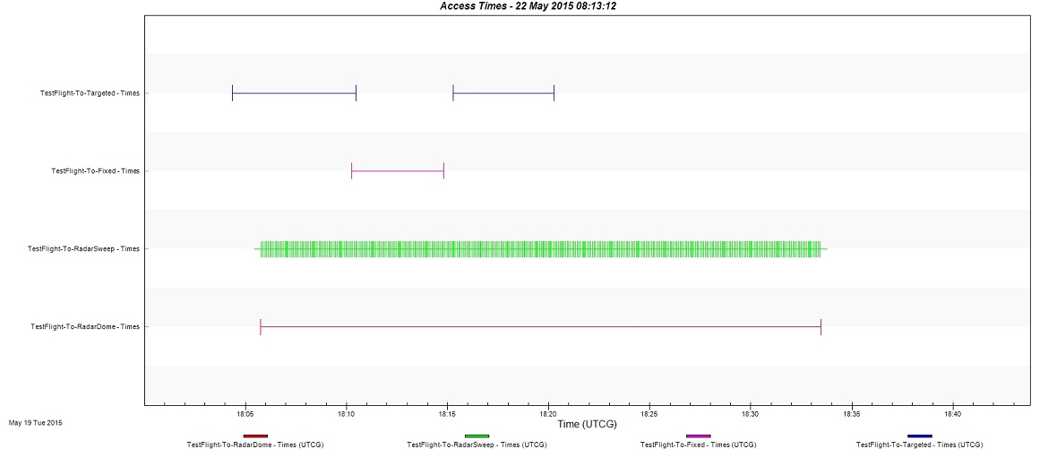
Multiple Access Graph
This graph shows you when each Sensor object accesses TestFlight. Your view may be different.
Saving Your Work
- When you are finished, close the Access graph and the Access Tool.
- Save () your work.