STK Pro, STK Premium (Air), STK Premium (Space), or STK Enterprise
You can obtain the necessary licenses for this tutorial by contacting AGI Support at support@agi.com or 1-800-924-7244.
The results of the tutorial may vary depending on the user settings and data enabled (online operations, terrain server, dynamic Earth data, etc.). It is acceptable to have different results.
This tutorial requires version 12.9 of the STK software or newer to complete.
Capabilities covered
This lesson covers the following capabilities of the Ansys Systems Tool Kit® (STK®) digital mission engineering software:
- STK Pro
- Coverage
Problem statement
You require a quick and easy way to simulate three Earth-observing payloads in three different orbital planes. You need to know when any or all of the satellites' sensors can view the portion of the Earth's surface that falls between 60 degrees north and 60 degrees south latitude. Additionally, you would like to know if any areas of the Earth will be covered by two or three sensors simultaneously, during daylight hours, and if so, for how long. You need to determine the extent and quality of coverage provided by the three satellites.
Solution
Use the STK software's Coverage capability to model and analyze the quality and quantity of coverage provided by the Earth-observing payloads attached to the satellites in the three different orbital planes. Using this model, you will determine if, when, and for how long two or more of the satellites can survey the Earth's surface during daylight hours.
Upon completion of this tutorial, you will be able to:
- Understand a coverage grid
- Use constraints in a coverage grid
- Determine coverage assets
- Understand multiple Figure of Merit types
- Choose which data providers supply answers to your questions
- Create color contours pertaining to the coverage analysis in the 2D and 3D Graphics windows
- Use the Grid Inspector tool
Video guidance
Watch the following video. Then follow the steps below, which incorporate the systems and missions you work on (sample inputs provided).
Using the starter scenario
To speed things up and allow you to focus on the core aspects of this tutorial, a partially created scenario has been provided for you.
Opening the starter scenario
The starter scenario is included in your install.
- Launch the STK application (
 ).
). - Click
 Open a Scenario in the Welcome to STK dialog box.
 - Browse to <Install Dir>\Data\Resources\stktraining\VDFs.
- Select Coverage_GettingStarted.vdf.
- Click .
Saving the VDF as a scenario file
Save and extract the VDF data in the form of a Scenario folder. When you save a VDF in the STK application, it will save in its originating format. That is, if you open a VDF, the default save format will be a VDF (.vdf). If you want to save and extract a VDF as a scenario folder, you must change the file format by using the Save As feature. This will create a permanent scenario file complete with child objects and any additional files packaged with the VDF.
- Open the File menu when the starter scenario opens.
- Select Save As....
- Select the STK User folder in the navigation pane when the Save As dialog box opens.
- Select the Coverage_GettingStarted folder.
- Click .
- Select Scenario Files (*.sc) in the Save as type drop-down list.
- Select the Coverage_GettingStarted STK scenario file in the file browser.
- Click .
- Click in the Confirm Save As Dialog box to overwrite the existing scenario file in the folder and to save your scenario.
A scenario folder with the same name as the VDF was created for you when you opened the VDF in the STK application. This folder contains the temporarily unpacked files from the VDF.
When saving a VDF as a scenario folder, you should extract its contents to the scenario folder the STK application automatically creates for you in the STK User folder. See the
Save (![]() ) often during this lesson!
) often during this lesson!
Reviewing the starter scenario
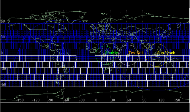
The starter scenario contains three previously defined satellites. Each satellite is equipped with a sensor used to model the field of view of the attached data collection instrument.
- Click on the 2D Graphics window to select it.
- Open the Window menu.
- Select Tile Vertically in the shortcut menu.
- Look at the objects in the scenario.
- Earth-observing payloads (Sensor objects) are attached to three different satellites.
- Shuttle is in a circular orbit with a 51.6 degree inclination.
- SunSync is in a Repeating Sun-synchronous orbit.
- TestSat is in a circular orbit with a 70 degree inclination.
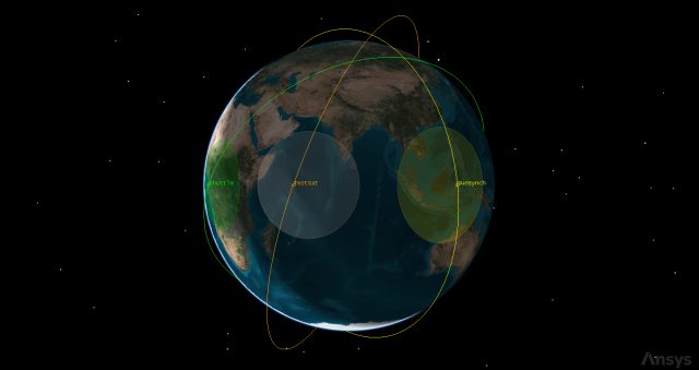
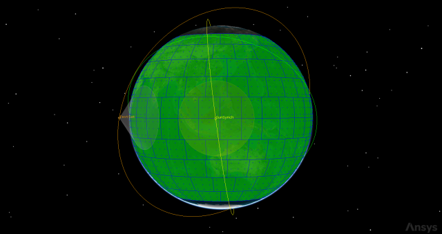
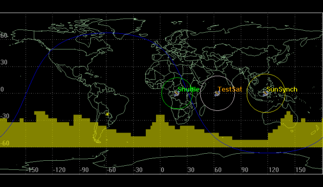
3D View: Three predefined orbits
The Earth-observing mission that these satellites are performing requires the Earth to be in sunlight in order for data collection to occur. You are only interested in the area on the surface of the Earth that falls between 60 degrees north latitude and -60 degrees south latitude.
Inserting a Coverage Definition object
The STK software's Coverage capability allows you to analyze the global or regional coverage provided by one or more assets (facilities, vehicles, sensors, etc.) while considering all accesses. To address area coverage capabilities, Coverage provides you with two STK object classes: Coverage Definition objects and Figure of Merit Objects. Before running a Coverage analysis, however, you must first insert a Coverage Definition object.
While you know what your region of interest is — the portion of the Earth's surface that falls between 60 degrees and -60 degrees latitude — you still need to tell the STK application to use that area as your region of interest. Insert a
- Bring the Insert STK Objects tool (
 ) to the front.
 - Select Coverage Definition (
 ) in the Select An Object To Be Inserted list.
 - Select the Insert Default () method in the Select A Method list.
- Click .
- Right-click on CoverageDefinition1 () in the Object Browser.
- Select Rename in the shortcut menu.
- Rename CoverageDefinition1 () Stereo_Cov.
Defining a coverage grid
Coverage analyses are based on the accessibility of assets (objects that provide coverage) and geographical areas. For analysis purposes, the geographical areas of interest are further refined using regions and points defined by the STK application. Points have specific geographical locations and are used in the computation of asset availability. Regions are closed boundaries that contain sets of points. The combination of the geographical area, the regions within that area, and the points within each region is called the
Specifying the Grid Area of Interest
Specific results are generated based on detailed access computations performed to user-defined grid points within an area of coverage set by the Grid Definition. The default Grid Definition type is set to Latitude Bounds. This definition results in a coverage region, called the
- Open Stereo_Cov's () Properties (
 ).
). - Select the Basic - Grid page when the Properties Browser opens.
- Enter the following values in the Grid Area of Interest panel:
| Option | Value |
|---|---|
| Min Latitude | -60 deg |
| Max Latitude | 60 deg |
Setting the grid resolution
While the area to be considered in the coverage analysis is specified by a set of regions within the defining bounds, the statistical data computed during a coverage analysis are based on a set of locations, or grid points, which span the coverage area. You can determine the spacing between grid points using the options in the
Finer grid resolutions typically produces more accurate results, but require additional computational time and resources.
- Enter 4 deg in the Lat/Lon field in the Point Granularity panel.
- Click to apply the changes and keep the Properties Browser open.
Choosing coverage graphics
You can define how the coverage grid is displayed in the 2D and 3D Graphics window using the Graphics Attributes properties for the Coverage Definition object. The fields on the
- Select the 2D Graphics - Attributes page.
- Select the Show Regions check box in the Grid panel.
- Click to apply the changes and keep the Properties Browser open.
Getting a better look
The sections and lines outlined on the globe represent coverage regions and individual points within those regions. The points have a specific geographical location and are used in the computation of assets available. Accessibility to a region is computed based on accessibility to the points within that region.
- Bring the 3D Graphics window to the front.
- Move around in the 3D Graphics window to get a good look at the coverage grid.
- Move around in the 3D Graphics window to get a good look at the north and / or south pole.
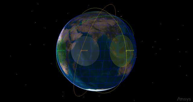
3D View: Stereo_Cov's grid display
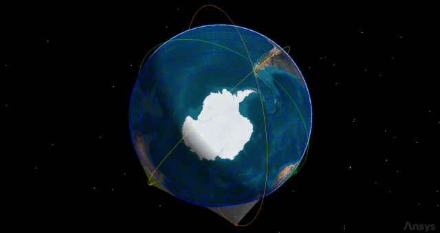
3D View: Stereo_Cov's grid extents
Notice that there is no grid covering either of these areas. When you limited the boundaries of your coverage region, the STK application excluded these areas from the grid.
Managing your resources
By default, the STK application is set to automatically recompute access every time an object on which the coverage definition depends (such as an asset) is updated. You will be computing access to a large area, which could take some time. In an effort to manage your resources more efficiently, turn off recomputing access automatically every time you make a change.
- Return to Stereo_Cov's () Properties ().
- Select the Basic - Advanced page.
- Clear the Automatically Recompute Accesses check box.
- Click to accept your changes and to close the Properties Browser.
Constraining your coverage
Your first objective is to determine what areas of the Earth, at some time in a 24 hour period, will be examined by at least one of the sensors during daylight hours. If coverage is based on access to every point in the grid, how will you ensure that the grid points are constrained based on the lighting conditions in that geographical area?
Once you have defined the grid area and resolution, you can customize the definition of points within the grid, by specifying a type of object or a specific object as a template for the points within the grid. The
Creating the constraints template
Since you want to constrain your analysis based on the lighting conditions on the ground, apply a
- Bring the Insert STK Objects tool () to the front.
- Insert a facility (
 ) object using the Insert Default () method.
 - Rename Facility1 () Const_Template.
Applying a Sun constraint
Any constraints or characteristics that you want to impose on points in the coverage grid must be applied to the template object. You can set a lighting constraint on Const_Template, which, once associated with the coverage definition, will be used by every point in the coverage grid.
- Open Const_Template's () Properties ().
- Select the Constraints - Active page.
- Click Add new constraints (
 ) in the Active Constraints toolbar.
 - Select Lighting in the Constraint Name list when the Select Constraints to Add dialog box opens.
- Click .
- Click to close the Select Constraints to Add dialog box.
- Look at the Lighting panel in the Constraint Properties panel.
- Click .
- Clear the Const_Template () check box in the Object Browser.
The default selection is Direct Sun (total sunlight). This is the constraint you need for your analysis.
The location and display of the constraints template is unimportant. You don't need to see the Facility object in either the 2D or 3D Graphics windows for it to be used analytically, so clearing it help keeps your scenario organized.
Associating the Sun constraint to the coverage grid
You have applied the appropriate constraint to the Const_Template Facility object, but you still need to associate that object with Stereo_Cov.
- Open Stereo_Cov's () Properties ().
- Select the Basic - Grid page when the Properties Browser opens.
- Click in the Grid Definition panel.
- Set the following options in the Grid Constraint Options dialog box:
- Select Const_Template in the Object Instance list.
- Click to close the Grid Constraint Options dialog box.
- Click .
| Option | Value |
|---|---|
| Reference Constraint Class | Facility |
| Use Object Instance | Selected |
Identifying your coverage assets
You've defined and constrained the area within which you'd like to analyze coverage. The next step is to identify your assets. Coverage assets specify which objects, or assets in the scenario, will be used to provide coverage over the specified region.
The Earth-observing payload attached to each satellite (Shuttle, SunSync,and TestSat) are modeled using a Sensor object in this scenario; therefore, the sensors attached to each satellite will be your assets
- Select the Basic - Assets page.
- Expand (
 ) each Satellite object (
 ).
). - Hold down the Ctrl key and
 ) objects.
 - Click .
- Click .
The display in the Assets list will change to visually indicate which objects in the scenario have been assigned as assets.
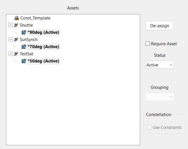
Assigned assets for Stereo Cov
Using the Compute Accesses tool
The ultimate goal of coverage is to analyze accesses to an area by using assigned assets and applying necessary limitations upon those accesses. You have a coverage definition (Stereo_Cov), which covers the surface of the Earth between 60 degrees and -60 degrees and you've assigned assets (the Earth-observing payload on each satellite) that will provide access to that area-of-interest. Now that the coverage definition object is defined and properly contained, access periods to the coverage area can be computed to determine the availability of an asset or set of assets that satisfy all geometric, lighting, temporal and other specified constraints. Use the Compute Accesses tool to compute accesses for the coverage definition.
- Bring the 2D Graphics window to the front.
- Right-click on Stereo_Cov () in the Object Browser.
- Select CoverageDefinition in the shortcut menu.
- Select Compute Accesses in the CoverageDefinition submenu.
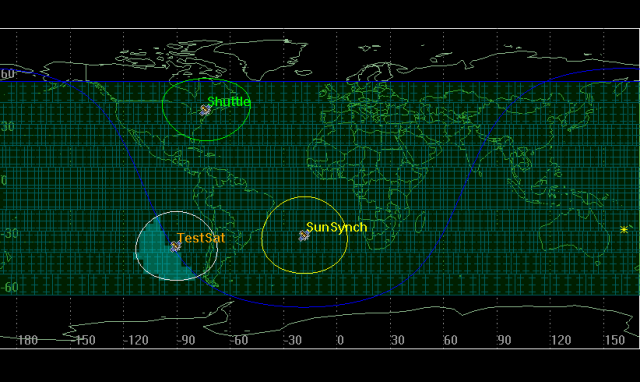
Coverage graphics display in the 2D Graphics window while coverage is being computed. When you compute coverage, all access calculations between the coverage assets (all three Sensor objects) and the coverage area (Stereo_Cov) are computed. A Progress Bar will display in the STK application's Status Bar which displays the Coverage computational progress (%).
For larger-scale calculations, consider computing the accesses for coverage in parallel using multiprocessing. This can be done using multiple cores with Compute Accesses in Parallel. When you choose this option, the STK application saves the current state of your scenario to a temporary VDF; worker processes are started on the local machine or on the cluster machine depending on your configuration and then the results are sent back to the STK application.
If you select white as the color for the coverage definition, you will not see any computational progress.
2D View: Coverage computation display
Defining the quality of coverage with a simple coverage Figure of Merit
While the Coverage Definition object defines the problem, a
To evaluate coverage quality, you will first need to set basic parameters that determine the way in which quality is computed. This involves choosing the method for evaluating the quality of coverage provided, setting measurement options, and identifying the criteria needed to achieve satisfactory coverage.
Measuring simple coverage
Evaluate the quality of coverage within your coverage region using a simple coverage type Figure of Merit object.
- Insert a Figure of Merit (
 ) object using the Insert Default () method.
 - Select Stereo_Cov () in the Select Object dialog box.
- Click .
- Rename FigureOfMerit1 () Simple_Cov.
The STK application creates a simple coverage figure of merit by default. Since you will be evaluating simple coverage, there is no need to change SimpleCov's properties.
Configuring static coverage graphics
Graphics are used to represent the static and dynamic value of simple coverage. When displaying static graphics, grid points are highlighted if they are covered by at least one asset at any time during the analysis time period. The figure of merit display shows you where, during daylight hours, you have coverage by at least one asset during the coverage interval.
- Bring the 3D Graphics window to the front.
- Move around the 3D Graphics window to view the coverage quality.
3D View: Simple coverage quality for Stereo_Cov
In this case, the entire coverage region is shaded here in green. Your color could be different. This tells you that, at some point during the 24 hour analysis interval, each point in your coverage region did have access to at least one asset during daylight hours.
Viewing dynamic coverage graphics
Look at coverage graphics in the 2D Graphics window. In the 2D Graphics window you can see the entire globe as a flat map, whereas in the 3D Graphics window, the sunlit portion of the globe may be hidden when accesses occur.
- Bring the 2D Graphics window to the front.
- Click Decrease Time Step (
 ) in the Animation toolbar and set the Time Step to 10.00 sec.
 - Click Start (
 ) to animate your scenario.
 - Click Reset (
 ) when you are finished.
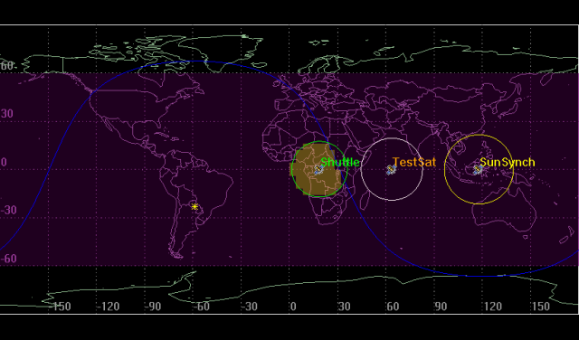
2D View: Simple coverage quality dynamic display
The solar terminator as well as the subsolar point have already been enabled for you in the window's
Each of your assets has access for some portion of the 24 hour period, but how many of those assets have coverage in the same area simultaneously during daylight hours? A second Figure of Merit object can be used to answer that very question.
Cleaning up the 2D and 3D Graphics windows
In an effort to minimize clutter and more clearly visualize periods of access, remove the grid from the visualization windows and focus on the coverage quality display.
- Open Stereo_Cov's () Properties ().
- Select the 2D Graphics - Attributes page.
- Clear the Show Regions check box.
- Clear the Show Points check box.
- Click .
- Clear the check box beside Simple_Cov () in the Object Browser.
Defining the quality of coverage with N Asset Coverage
Insert a second Figure of Merit (![]() ) object that will analyze the quality of coverage based on the number of available assets, called an N Asset Coverage Figure of Merit.
) object that will analyze the quality of coverage based on the number of available assets, called an N Asset Coverage Figure of Merit.
Inserting a new Figure of Merit object
Add a new Figure of Merit object to Stereo_Cov.
- Insert a Figure of Merit () object using the Insert Default () method.
- Select Stereo_Cov () in the Select Object dialog box.
- Click .
- Rename FigureofMerit2 () NAsset_Cov.
Using N Asset Coverage
Set the coverage definition properties to utilize N Asset Coverage.
- Open NAsset_Cov's () Properties ().
- Select the Basic - Definition page when the Properties Browser opens.
- Set the following in the Definition panel:
- Click .
| Option | Value |
|---|---|
| Type | N Asset Coverage |
| Compute | Maximum |
Selecting maximum computes the maximum number of assets available over the entire coverage interval. In this case, for every grid point the static value of the FOM is the maximum number of sensors (assets) simultaneously providing coverage during the analysis interval.
Getting a better look
View the coverage graphics in the 2D Graphics window.
- Bring the 2D Graphics window to the front.
- Review the quality of coverage.
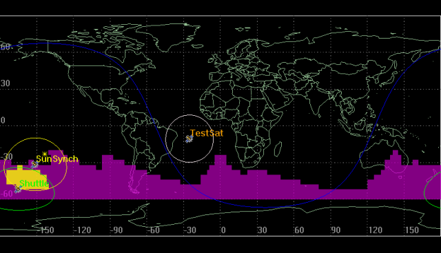
2D View: NAsset FOM coverage graphics
Choosing the satisfaction criterion
You can restrict NAsset_Cov's behavior so that the STK application only applies the graphical properties when a chosen
- Return to NAsset_Cov's () Properties ().
- Set the following in the Satisfaction panel:
- Click .
| Option | Value |
|---|---|
| Enable | Selected |
| Satisfied If | At Least |
| Threshold | 2 |
The application of the Satisfaction criterion determines which grid points are graphically highlighted in the dynamic and static graphics. In this case, you want the Satisfaction Criterion to be that at least two (the selected threshold) of the assets (sensors) have access to a point in the grid simultaneously during daylight hours.
Decreasing the translucency
To ensure the graphics display brightly against the globe, you can decrease the percent translucency on the Figure of Merit's
- Select the 2D Graphics - Animation page.
- Enter 20 in the % Translucency field in the Show Points As panel.
- Click .
- Select the 2D Graphics - Static page.
- Enter 20 in the % Translucency field in the Show Points As panel.
- Click .
Getting a better look
Adding the satisfaction criteria has greatly reduced your area of coverage as evidenced by the 2D and 3D Graphics display.
- Bring the 3D Graphics window to the front.
- Bring the 2D Graphics window to the front.
- Click Start () to animate your scenario.
- Click Reset () when you are finished.
3D View: NAsset FOM satisfaction graphics
Your colors might be different from the above image.
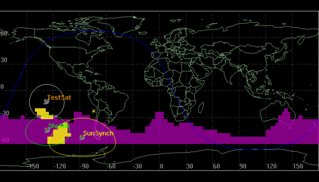
2D View: NAsset FOM satisfaction graphics
Notice that, as the scenario animates, a single sunlit sensor no longer shows dynamic coverage graphics. With the satisfaction criteria applied, you only see dynamic coverage graphics if there is double or triple coverage.
Graphing coverage by latitude
Create a Coverage By Latitude graph to confirm what you are seeing in the 2D Graphics window.
- Right-click on Stereo_Cov () in the Object Browser.
- Select Report & Graph Manager... (
 ) in the shortcut menu.
 - Clear the Show Reports check box in the Styles list of the Report & Graph Manager.
- Select the Coverage By Latitude (
 ) graph in the Installed Styles (
 ) folder.
 - Click .
Understanding the coverage by latitude data provider
The coverage by latitude data provider reports coverage for each latitude in the selected range (-60 degrees to 60 degrees), at intervals depending on the selected resolution. A point is considered to be covered if it has access to one or more of the assigned assets. The reported values for each latitude are the average value for all grid points at that latitude.
- Review the Coverage by Latitude graph.
- Close the Coverage by Latitude graph.
- Click to close the Report & Graph Manager.
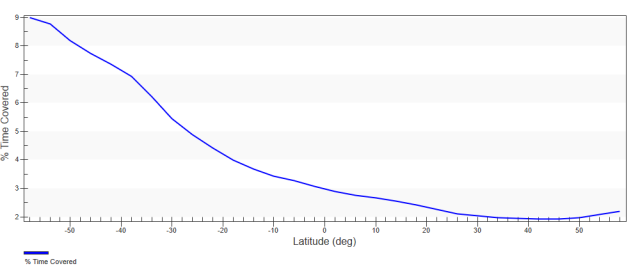
Graph: Stereo Cov percent of time covered by latitude
The graph coincides with what you see in the 2D and 3D Graphics windows. As your latitude increases, your coverage decreases.
Visualizing accumulated coverage
Your analysis up to this point has illustrated instantaneous coverage. You would also like to determine what areas, at some time during the day, had single, double, or triple coverage.
Setting the accumulation options
The accumulation options for animation graphics allow you to control the sense and persistence of the animation graphics. By default, the STK application is set to highlight grid points that meet the satisfaction criteria at the current time. When you change the accumulation value to Up to current time, grid points that have met the satisfaction criterion based on the dynamic definition of the figure of merit from the start time to the current time are highlighted during animation. This can help you determine not only where you have the best coverage but also when you have the best coverage.
- Open NAsset_Cov's () Properties ()
- Select the 2D Graphics - Animation page when the Properties Browser opens.
- Open the Show drop-down list in the Accumulation panel.
- Select Up to current time.
- Click .
Viewing up to current time in the 2D Graphics window
Because you made minimal changes to the 2D Graphics properties for the NAsset_Cov (![]() ), by default both static and animation graphics display in the 2D and 3D Graphics windows. Whenever an assigned asset passes through the coverage area it leaves a footprint that indicates where the quality criteria (at least two assets) was met at a specific point in time.
), by default both static and animation graphics display in the 2D and 3D Graphics windows. Whenever an assigned asset passes through the coverage area it leaves a footprint that indicates where the quality criteria (at least two assets) was met at a specific point in time.
- Bring the 2D Graphics window to the front.
- Click Start () to animate your scenario.
- Click Reset () when you are finished.
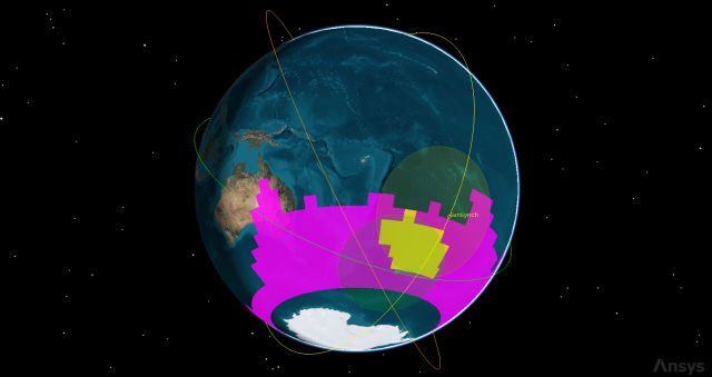
2D View: NAsset FOM up to current coverage
In the above image, the pink shading (the static graphics) shows the sum of what has been covered by at least two assets at some time during the entire coverage interval. The yellow shading (animation graphics) shows how coverage is accumulated. When you animate the scenario, the animation graphics will accumulate as additional areas of the Earth are covered by at least two assets over time until they match the total static coverage for the coverage interval. Since the static coverage is the sum of the accumulated coverage it will eventually equal or add up to the static graphics.
Understanding contour graphics
You can specify how levels of coverage quality display in both the 2D and 3D Graphics windows using
Before you display contour graphics, turn off the display of the Animation graphics for NAsset_Cov.
- Return to NAsset_Cov's () Properties ().
- Select the 2D Graphics - Animation page.
- Clear the Show Animation Graphics check box.
- Click .
Creating static contours
Static Contour levels display coverage data for all points based on evaluation over the entire coverage interval (in this case the analysis period).
- Select the 2D Graphics - Static page.
- Select the Show Contours option in the Display Metric panel.
- Click in Level Attributes panel.
- Enter the following values in the Level Adding panel:
- Click .
| Option | Value |
|---|---|
| Add Method | Start, Stop, Step |
| Start | 1 |
| Stop | 3 |
| Step | 1 |
Selecting the contour colors
Use a color ramp from red to blue for your coverage graphics. The Color Ramp method applies a spectrum pattern with selected start and end colors.
- Enter the following values in the Level Attributes panel:
- Click .
| Option | Value |
|---|---|
| Color Method | Color Ramp |
| Start Color | Red |
| End Color | Blue |
Note that the Start Color corresponds to the first Level value under Level Attributes.
Creating an embedded legend for the 2D and 3D Graphics windows
A contour key, or
- Click in the Level Attributes panel.
- Click in the Static Legend for NAsset_Cov floating legend.
- Select the Show at Pixel Location check box in both the 2D Graphics Window and 3D Graphics Window panels in the Figure of Merit Legend Layout dialog box.
- Click to close the Figure of Merit Legend Layout dialog box.
- Close the Static Legend for NAsset_Cov floating legend window.
The
Viewing the legend
View the legend you just added to the 2D and 3D Graphics windows.
- Bring either the 2D or 3D Graphics window to the front.
- You should see the legend in either window.
Static contours legend for NAsset coverage
The map graphics will be colored according to the number of available assets as outlined in the static contours legend.
Selecting natural neighbor sampling
You would like a smoother effect for the contours in your 2D and 3D Graphics windows. You can to use the Natural Neighbor Sampling option to accomplish this.
- Return to NAsset_Cov's () Properties ().
- Select the 2D Graphics - Static page.
- Select the Natural Neighbor option in the Contour Interpolation (points must be filled) panel.
- Click .
This option is not valid for these Coverage Definition types: Latitude Line, Longitude Line, and Custom Boundary.
Getting a better look
Color is applied smoothly over all points in the grid to differentiate contour levels. If you choose the Natural Neighbor Sampling, the value of the Figure of Merit is determined for each screen pixel within the coverage area using a natural neighbor interpolation algorithm based on the computed values of the Figure of Merit at the grid points. In the case of discreet figures of merit, interpolated values are rounded to the nearest integer. View the changes in both the 2D and 3D Graphics windows.
- Bring the 2D Graphics window to the front.
- Review the contours.
- Bring the 3D Graphics window to the front.
- Review the contours.
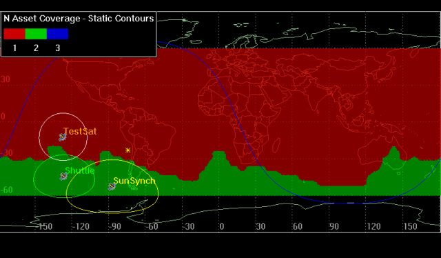
2D View: NAsset FOM static contours display
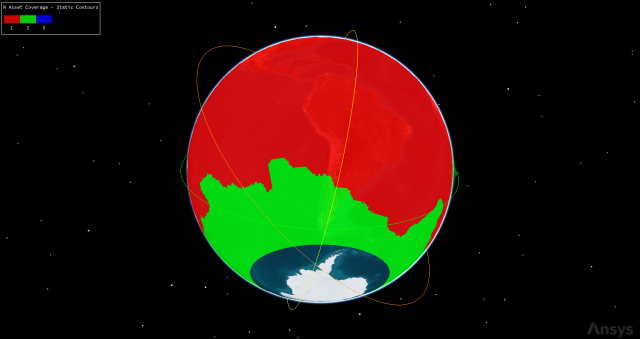
3D View: NAsset FOM static contours display
Creating dynamic contours
The static contour display tells you where you have access to at least one (red), two (green), or three (blue) assets at some point during the entire coverage interval. Take contours a step further. Display contours that will tell you how many assets you have access to based on the scenario time.
- Return to NAsset_Cov's () Properties ()
- Select the 2D Graphics - Static page.
- Clear the Show Static Graphics check box.
- Select the 2D Graphics - Animation page.
- Select the Show Animation Graphics check box.
- Select the Show Contours option in the Display Metric panel.
- Click in the Level Attributes panel.
- Click to confirm.
- Select the Natural Neighbor option in the Contour Interpolation (points must be filled) panel.
- Click .
Selecting Copy Static Levels ensures that the same contour levels and colors are used for both static and animation graphics.
Getting a better look
As your scenario animates areas in the coverage grid that have access to all three assets will be blue, the areas with double coverage will be green, and those with single coverage will be red.
- Bring the 2D Graphics window to the front.
- Click Start () to animate your scenario.
- Click Reset () when you are finished.
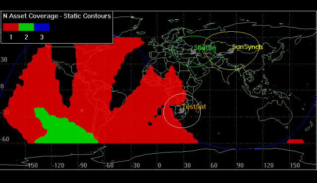
2D View: NAsset dynamic contours display
Contour graphics have shown you that you have coverage from one and two assets at various times throughout your coverage analysis, but how long do you have that coverage, and exactly where? You can use yet another type of Figure of Merit object to help answer that very question.
Removing NAsset_Cov's graphics
Before you create another Figure of Merit object, turn NAsset_Cov's graphics off, so that they don't interfere with the coverage quality display of the new Figure of Merit object.
- Clear the check box next to NAsset_Cov () in the Object Browser.
Using a Coverage Time Figure of Merit object
A
Inserting a third Figure of Merit object
Add a new Figure of Merit object to gauge Coverage Time.
- Insert a Figure of Merit () object using the Insert Default () method.
- Select Stereo_Cov () in the Select Object dialog box.
- Click .
- Rename FigureOfMerit3 () Cov_Time.
Measuring coverage time
Set the Figure of Merit type to Coverage Time.
- Open Cov_Time's () Properties ().
- Select the Basic - Definition page when the Properties Browser opens.
- Set the following in the Definition panel.
- Click .
| Option | Value |
|---|---|
| Type | Coverage Time |
| Compute | Total Time Above |
| Min # Assets | 2 |
The Total Time Above option computes the amount of time (over the entire coverage interval) during which a point is covered by at least the minimum number of assets specified.
Decreasing the translucency
To ensure the graphics display brightly against the globe, you need to decrease the percent translucency.
- Select the 2D Graphics - Static page.
- Enter 20 in the % Translucency field in the Show Points As panel.
- Click .
Getting a better look
View the coverage time graphics in the 2D Graphics window.
- Bring the 2D Graphics window to the front.
- Move around to see how the coverage over the globe.
2D View: Cov Time FOM graphics display
Reporting coverage time
Cov_Time's display shows that you have at least two assets viewing parts of the southern latitudes over the entire coverage interval. But what are the maximum, minimum, and average values over the entire coverage region? Use a
- Right-click on Cov_Time () in the Object Browser.
- Select Report & Graph Manager... () in the shortcut menu.
- Select the Show Reports check box in the Styles panel in the Report & Graph Manager.
- Clear the Show Graphs check box.
- Select the Grid Stats (
 ) report in the Installed Styles () folder .
 - Click .
- Note the minimum (e.g. 0.000 seconds), maximum (e.g. ~1697 seconds) and average (e.g. ~70 seconds) values for Cov_Time to help you define your contour levels.
- Close the report and the Report & Graph Manager.
Creating coverage time contours
Now that you have the values for your coverage time, you can use them to set the intervals for Cov_Time's contour graphics.
- Return to Cov_Time's () Properties ().
- Select the 2D Graphics - Static page.
- Select the Show Contours option in the Display Metric panel.
- Click in the Level Attributes panel.
- Set the following values in the Level Adding panel:
- Click .
| Option | Value |
|---|---|
| Add Method | Start, Stop, Step |
| Start | 100 sec |
| Stop | Round down to nearest 100 below the Maximum (sec) value found in the Grid Stats report (e.g. 1600 sec) |
| Step | 250 sec |
Any times under 100 seconds will show no color in both the 2D and 3D Graphics windows. Any times above 1600 seconds will show the end color.
Selecting the contour colors
Adjust the color ramp options for your contours.
- Enter the following values in the Level Attributes panel:
- Select the Natural Neighbor option in the Color Interpolation (points must be filled) panel.
- Click .
| Option | Value |
|---|---|
| Color Method | Color Ramp |
| Start Color | Red |
| End Color | Blue |
Creating an embedded legend for the 2D and 3D Graphics windows
As before, add a legend to your 2D and 3D Graphics windows.
- Click in the Level Attributes panel.
- Click in the Static Legend for Cov_Time floating legend.
- Select the Show at Pixel Location check box in both the 2D Graphics Window and 3D Graphics Window panels in the Figure of Merit Legend Layout dialog box.
- Enter Coverage Time (seconds) in the Title field in the Text Options panel.
- Enter 0 in the Number Of Decimal Digits field.
- Enter the following values in the Range Color Options panel:
- Click to close the Figure of Merit Legend Layout dialog box.
- Close the Static Legend for Cov_Time floating legend.
- Click to close the Properties Browser.
| Option | Value |
|---|---|
| Max Color Squares per Row | 40 |
| Color Squares Width (pixels) | 50 |
| Color Square Height (pixels) | 20 |
Getting a better look
View your contours and legends in the 2D and 3D Graphics windows.
- Bring the 2D Graphics window to the front.
- Bring the 3D Graphics window to the front.
- Move around to see how the contours cover the globe.
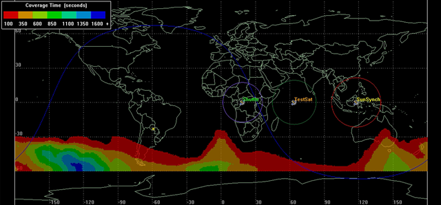
2D View: Cov Time FOM static contour display with legend
The legend is now embedded in the 2D map display for easy reference. The map graphics will be colored according to the length of time that assets are available as outlined in the static contours legend.
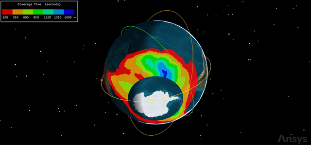
3D View: Cov Time FOM static contour display with legend
Reporting coverage time by grid point
The contours display provides a general overview of when you have coverage by two or more assets for how long, and the animation time can serve as a reference for when you the extended periods of coverage occur. To get a more thorough outline of the exact length of time each point in the grid is covered by two or more assets, create a report of values by grid point.
Creating a Value by Grid Point report
A Value by Grid Point report returns a detailed list which includes the geodetic coordinates of each point in the grid, and the length of time that each point is covered by at least two assets (the minimum assets specified in the FOM definition) while in direct sunlight (the constraint imposed on the grid points using the Const_Template facility object).
- Right-click on Cov_Time () in the Object Browser.
- Select Report & Graph Manager... () in the shortcut menu.
- Select the Value By Grid Point () report in the Installed Styles () list.
- Click .
- Review the report.
- Are there any grid points in the southern hemisphere that have values?
- Which latitude / longitude has the highest value (most time covered)?
- When you finish, close the Value By Grid Point report.
- Click to exit the Report & Graph Manager.
Using the Grid Inspector tool
The
Preparing the 2D Graphics window for the Grid Inspector tool
In order to use the Grid Inspector tool, you must show the grid points in the 2D Graphics window.
- Open Stereo_Cov's () Properties ().
- Select the 2D Graphics - Attributes page when the Properties Browser opens.
- Select the Show Regions check box in the Grid panel.
- Select the Show Points check box.
- Click .
Opening the Grid Inspector tool
Open the Grid Inspector tool for Cov_Time.
- Bring the 2D Graphics window to the front.
- Right-click on Cov_Time () in the Object Browser.
- Select FigureOfMerit in the shortcut menu.
- Select Grid Inspector... (
 ) in the FigureOfMerit submenu.
Obtaining region data
Inspect a region using the Grid Inspector tool.
- Open the Action drop-down list.
- Choose Select Region.
- Bring the 2D Graphics window to the front.
- Click anywhere in the 2D Graphics window where there is coverage.
- Read the information in the Messages field concerning the selected region.
Changing the Figure of Merit
There are several
- Clear the Cov_Time () check box in the Object Browser.
- Select the NAsset_Cov () check box in the Object Browser.
- Open NAsset_Cov's () Properties ().
- Select the 2D Graphics - Animation page when the Properties Browser opens.
- Clear the Show Animation Graphics check box.
- Click .
- Select the 2D Graphics - Static page.
- Select the Show Static Graphics check box.
- Click .
Creating a Region Figure of Merit report
The
- Bring the Grid Inspector tool to the front.
- Click .
- Select NAsset_Cov () in the Select Object dialog box.
- Click .
- Open the Action drop-down list.
- Choose Select Region.
- Click on a grid point anywhere in the 2D Graphics window where there is coverage.
- Click in the Reports panel.
- Review the data in the report.
- Close the report when you are finished.
Narrowing the focus to just one point
Narrow the focus to an actual point.
- Open the Action drop-down list.
- Choose Select Point.
- Bring the 2D Graphics window to the front.
- Click on a grid point where there is coverage.
- Read the information in the Messages field concerning the selected point.
- Feel free to continue to click various points in the Coverage results.
- Feel free to create any report or graphs.
- Close the Grid Inspector tool when you are done.
The Messages field displays, among other information, the value of the Total Time covered by 2 or more assets for that point.
Saving your work
Close out your work and save your scenario.
- Close any open reports, properties and the Report & Graph Manager.
- Save (
 ) your work.
Summary
You learned how to use a Coverage Definition object to include defining the grid, creating a direct sun constrained template object and applying that to the grid. You learned how to choose coverage assets. You looked at multiple Figures of Merit setups and analyzed simple , number of assets and coverage time coverage. You used multiple data providers to analyze your grid. Using the data, you created color contours that corresponded to the data. Finally, you used the Grid Inspector tool to focus analysis in selected regions and points inside of the coverage grid.