Astrogator Lambert Profile LEO to GEO
STK Premium (Space) or STK Enterprise
You can obtain the necessary licenses for this tutorial by
This tutorial requires STK 12.4 or later and is not compatible with earlier versions of the STK software.
The results of the tutorial may vary depending on the user settings and data enabled (online operations, terrain server, dynamic Earth data, etc.). It is acceptable to have different results.
Capabilities covered
This lesson covers the following capabilities of the Ansys Systems Tool Kit® (STK®) digital mission engineering software:
- STK Pro
- Astrogator
Problem statement
Engineers and operators need to understand the solution space for transfer arcs. Lambert's problem examines:
- The transfer arc between two position vectors
- The time of flight
This is useful for rendezvous operations, targeting, and preliminary orbit determination. Another common application is interplanetary missions (see the Mars Probe lesson). In this example, you will explore the transfer arc from low Earth orbit (LEO) to geostationary orbit (GEO). Because you can design an arc with different times of flight, energy, and Delta-V, there are many transfer solutions available to you.
Solution
Use the STK/Astrogator® capability to explore the solution space of transfers from LEO to GEO. First, you will examine the feasibility and Delta-V of a set of Lambert Profile transfers for a fixed time of flight. Then you will use the Lambert Search Profile, which finds the most fuel efficient solution in a range of times of flight, to then iterate to a full force solution.
What you will learn
Upon completion of this tutorial, you will be able to:
- Solve transfer arcs with the Lambert Profile
- Explore the solution space with the Lambert solver
- Solve transfer arcs with the Lambert Search Profile
- Iterate to a full force solution
Video guidance
Watch the following video. Then follow the steps below, which incorporate the systems and missions you work on (sample inputs provided).
Creating a new scenario
Create a new scenario with a duration of four days.
- Launch STK (
 ).
). - Click Create a Scenario (
 ) in the Welcome to STK dialog box.
 - Enter the following in the STK: New Scenario Wizard:
- When you finish, click .
- When the scenario loads, click Save (
 ). STK creates a folder with the same name as your scenario.
 - In the Save As dialog box, verify the scenario name and location, and click .
| Option | Value |
|---|---|
| Name | Lambert_LEO_to_GEO |
| Start | 15 Nov 2021 17:00:00.000 UTCG |
| Stop | + 4 days |
Save (![]() ) often!
) often!
Creating a LEO satellite and a (close to) GEO satellite
Create satellites named LEO_Orbit and GEO_Orbit to represent the initial and final orbits for your transfer. If both the starting and ending orbits are circular, then there are several transfer trajectories with the same minimum fuel usage, so changing the grid search time step slightly in the Lambert Search Profile can lead to a different-looking trajectory with similar Delta-V.
Creating the LEO satellite
Insert a new baseline LEO Satellite object using the Orbit Wizard method.
- Using the Insert STK Objects Tool, insert a Satellite (
 ) object using the Orbit Wizard (
 ) method.
 - Set the Type to Orbit Designer in the Orbit Wizard dialog box.
- Make the following changes:
- Set all other values to 0.
- Click when done.
| Option | Value |
|---|---|
| Satellite Name | LEO_Orbit |
| Semimajor Axis | 7000 km |
| Inclination | 28.5 deg |
Creating the GEO satellite
Next, create a reference GEO satellite.
- Insert a Satellite () object using the Orbit Wizard () method.
- Set the Type to Orbit Designer in the Orbit Wizard dialog box.
- Make the following changes:
- Set all other values to 0.
- Click when done.
- Look in the 3D Graphics window and adjust the view with your mouse until you see the two satellite orbits.
| Option | Value |
|---|---|
| Satellite Name | GEO_Orbit |
| Semimajor Axis | 42000 km |
| Inclination | 0 deg |
| Eccentricity | 0.05 |
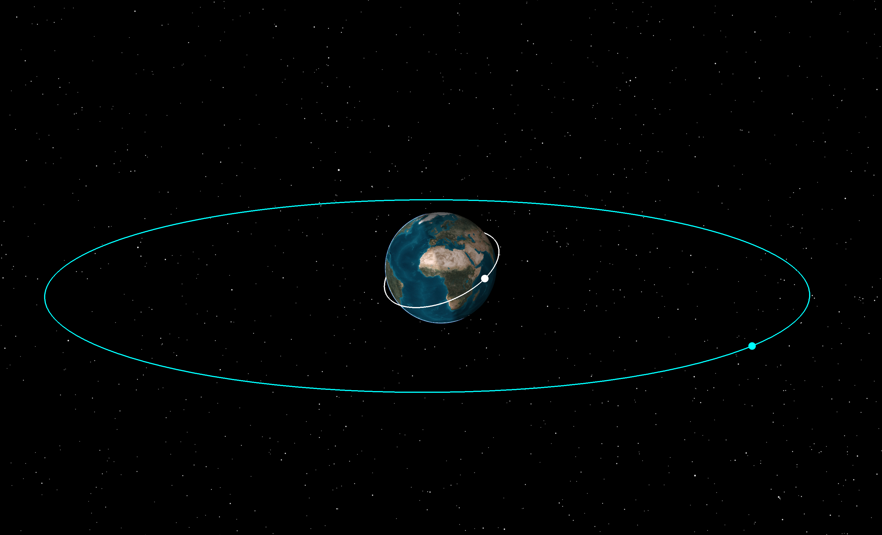
3D view of the LEO and GEO satellite orbits
Exploring an initial Lambert Profile solution
In this section, you will utilize the Lambert Profile to find a two-day transfer trajectory from the LEO orbit of the first satellite to the GEO orbit of the second satellite.
Adding a transfer satellite
You will use this satellite to model the transfer from LEO to GEO.
- Insert a Satellite () object using the Insert Default () method.
- Rename Satellite1 () TransferBasic.
- Open TransferBasic's () Properties (
 ).
). - Select the Basic - Orbit page.
- Set Propagator to Astrogator.
- Select the Propagate (
 ) segment in the Mission Control Sequence.
 - Click Delete Segment (
 ) in the MCS toolbar.
 - Click to confirm.
Setting the initial state of TransferBasic
Use the Initial State segment to define the initial conditions of your MCS, which are contained in the initial state of TransferBasic.
- Select Initial State (
 ) in the MCS.
 - Select the Elements tab.
- Use the settings of the LEO_Orbit satellite except for setting the true anomaly to 200 degrees. Set the following values:
- Click when done.
| Option | Value |
|---|---|
| Coordinate Type | Keplerian |
| Semi-major Axis | 7000 km |
| Inclination | 28.5 |
| True Anomaly | 200 deg |
Creating a target sequence
Use a Target Sequence as a structural element to define maneuvers and propagations in terms of the goals they are intended to achieve. In this part you will create the steps that the TransferBasic satellite will take to go from LEO to GEO. First, you need to create a target sequence that encompasses all the steps.
- Right-click on Initial State () in the MCS.
- Select Insert After... in the shortcut menu.
- Select Target Sequence (
 ) in the Segment Selection dialog box.
 - Click .
- Rename Target Sequence () Basic_Lambert.
Placing the initial maneuver in the target sequence
A basic Lambert sequence has two maneuver segments and a propagate segment between them. You will start the target sequence with a maneuver.
- Right-click on Basic_Lambert () in the MCS.
- Select Insert After... in the shortcut menu.
- Select Maneuver (
 ) In the Segment Selection dialog box.
 - Click .
- Click and drag the Maneuver () sequence so that it is nested beneath Basic_Lambert ().
Adding a Propagate segment
After the first maneuver, the TransferBasic satellite is in an intermediate orbit. This next segment will have the satellite fly in that orbit for some time.
- Right-click on Maneuver () in the MCS.
- Select Insert After... in the shortcut menu.
- Select Propagate () in the Segment Selection dialog box.
- Click .
Adding another maneuver
You will need a second maneuver to move the TransferBasic satellite into a GEO orbit.
- Right-click on Propagate () in the MCS.
- Select Insert After... in the shortcut menu.
- Select Maneuver () in the Segment Selection dialog box.
- Click .
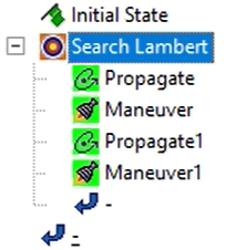
- Make sure the segments appear as in the following figure:
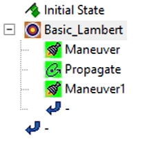
The Basic Lambert target sequence
Selecting the propagator
For the basic Lambert Profile, you want to use a simple force model, so set the Propagate segment to model Earth as a point mass.
- Select Propagate () in the MCS.
- Click the Propagator ellipsis(
 ) on the right.
 - Select Earth Point Mass (
 ) in the Select Component dialog box..
 - Click .
Building a Lambert profile
You have all the required steps in your target sequence to get from LEO to GEO. Now you will change the properties of the target sequence to use a Lambert Profile as your method for computing the sequences.
- Select Basic_Lambert () in the MCS.
- Remove the Differential Corrector by clicking Delete Profile () in the Profiles panel on the right.
- Click to confirm delete.
- Click New... (
 ) in the Profiles panel.
 - Select Lambert Profile () (not Lambert Search Profile) in the New... dialog box.
- Click .
- Click Properties... () for the Lambert Profile in the Profiles toolbar.
- Set the following:
- Click when done.
| Parameter | Setting |
|---|---|
| Time of Flight | 2 day |
| Target Coordinate Type | Keplerian |
| Semimajor Axis | 42000 km |
| Eccentricity | 0.05 |
| True Anomaly | 6.869 deg
See the section "Determining the true anomaly" later in the tutorial for how to compute this value. |
| Calculate Second Maneuver at Destination | Selected |
| Write Initial Delta-V to Maneuver | Selected |
| Write Duration to Propagate | Selected |
| Disable Non-LambertDuration Stopping Conditions in Propagate Segment | Selected |
| Write Final Delta-V to Maneuver | Selected |
Computing the transfer
You now have the segments in place, and the target sequence is set to use the basic Lambert method. Now run the entire mission control sequence to compute the maneuvers.
- Select Run active profiles in the Action drop-down list.
- Click Run Entire Mission Control Sequence (
 ) in the MCS toolbar.
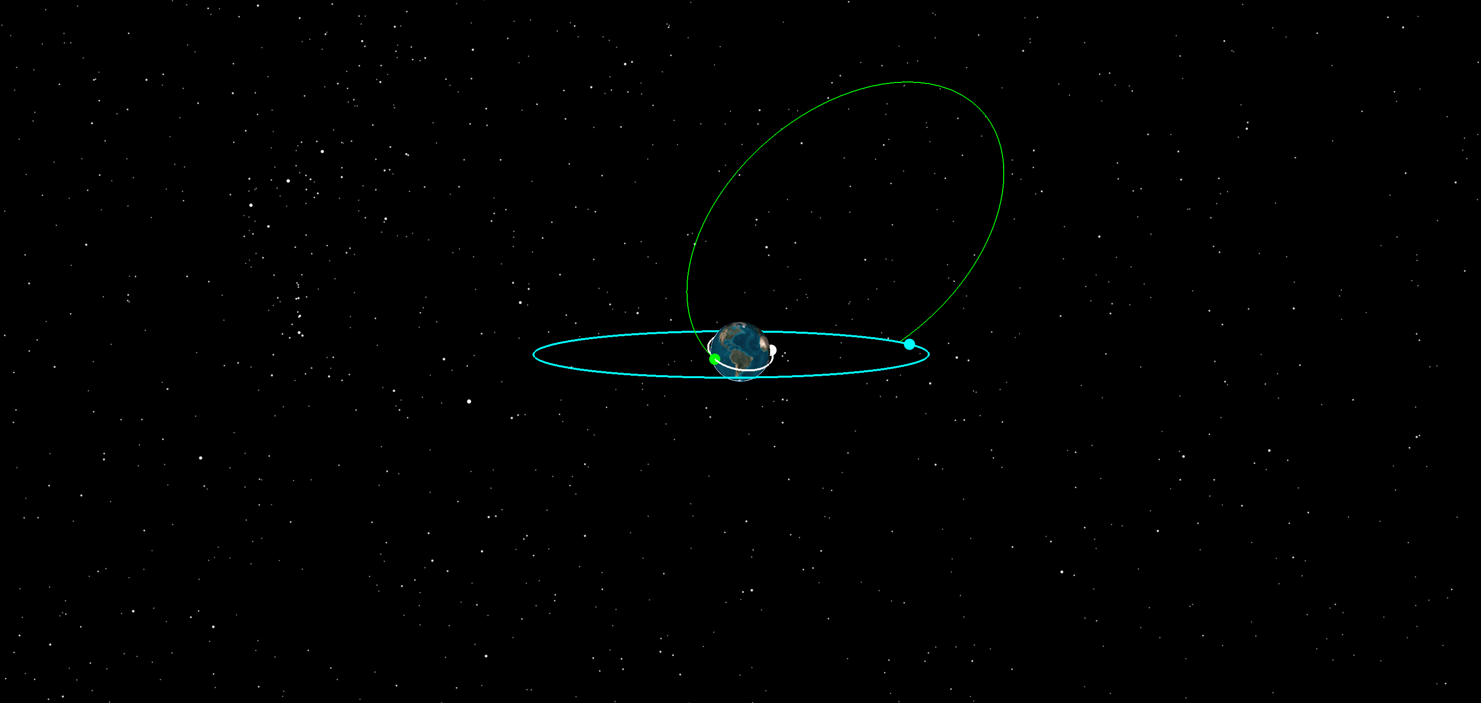
 - Examine the 3D Graphics window.
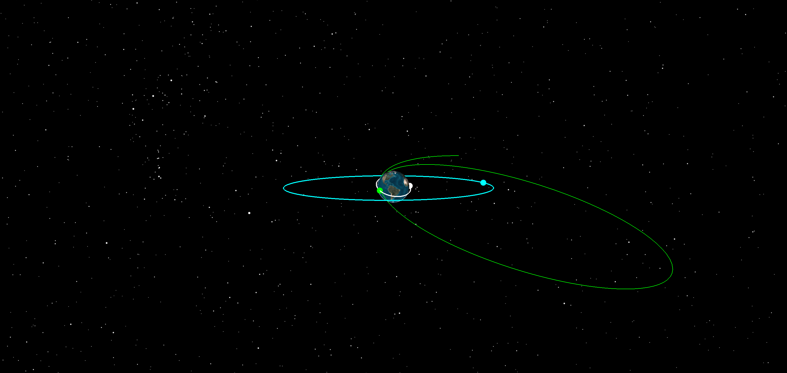
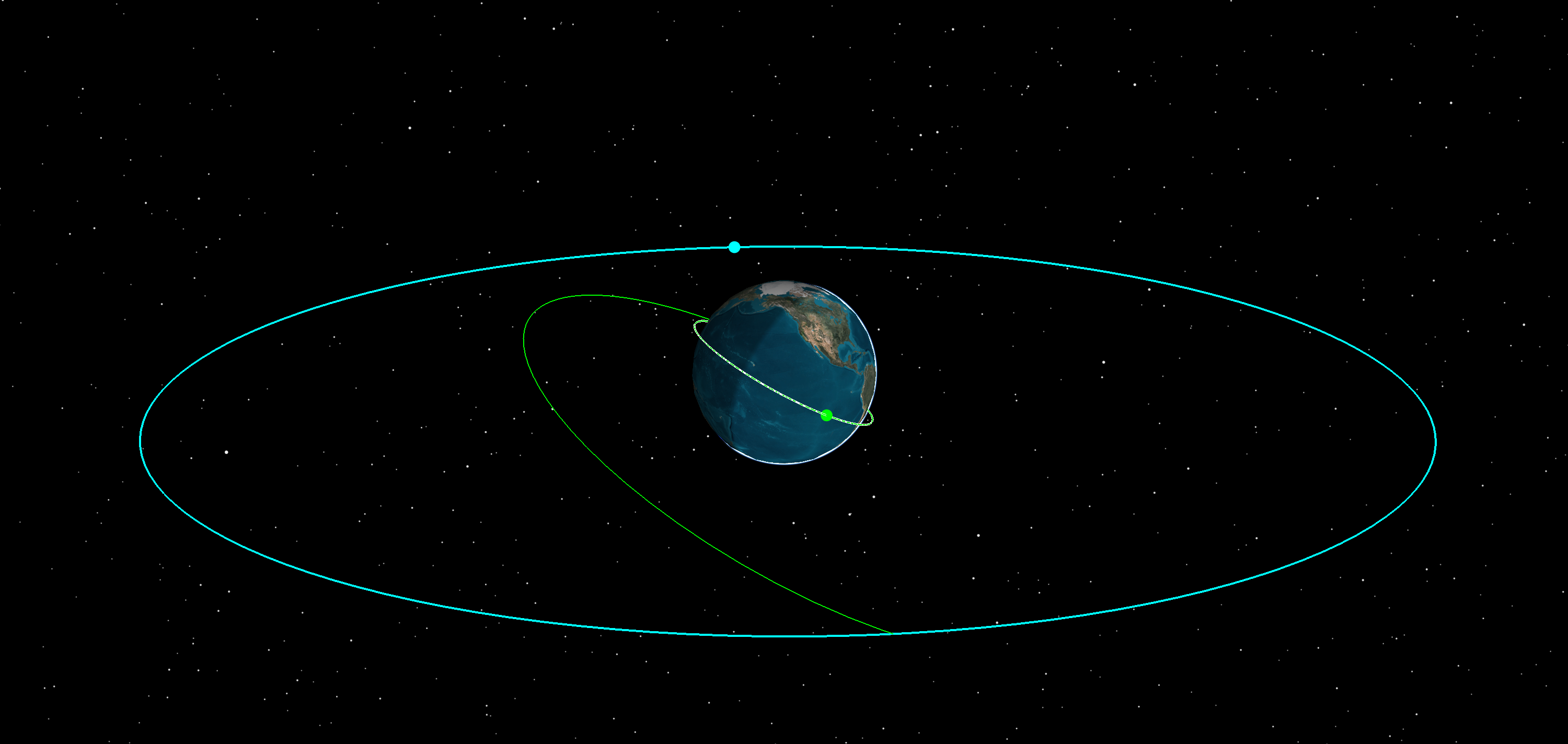
The Lambert arc goes to the GEO orbit. This is possible because you changed the propagator to Earth Point Mass. If you left the propagator as Earth Default High Fidelity v13, the transfer arc would end close to the GEO Orbit, but it would not intersect the final orbit exactly. Also, because of the long two-day fixed time of flight, the transfer geometry is quite skewed.
![]()
Transfer arc for the initial basic Lambert run
Determining the true anomaly (optional)
You can determine the true anomaly by generating a report of the Keplerian orbital elements for the GEO_Orbit satellite and looking at the True Anomaly value for the specified time of flight (2 days, or 172,800.000 EpSec).
Creating a true anomaly report
Create a new custom report style for your report.
- Open the Report & Graph Manager (
 ) from the Analysis menu.
 - On the left, make sure the Object Type is Satellite.
- Select GEO_Orbit ().
- Select the My Styles folder in the Styles panel on the right.
- Click Create new report style (
 ) in the Styles toolbar.
 - Name this report True_Anomaly and remain in the rename mode.
- Select the Enter key.
Adding parameters to the report
Select the data provider elements for your report.
- When True_Anomaly's Properties open, select the Content page.
- Expand (
 ) the Astrogator Values () data provider in the Data Providers panel.
 - Expand () the Keplerian Elems (
 ) data provider group.
 - Select and move (
 ) the following data provider elements (
 ) to the Report Contents panel:
- Time
- True Anomaly
- Select Time in the Report Contents panel.
- Click at the bottom.
- Clear the Use Defaults check box.
- Select Epoch Seconds (EpSec) in the New Unit Value panel.
- Click to close the Units dialog box.
- Click to apply the changes and close the True_Anomaly Report Style properties.
Generating the True_Anomaly report
With your custom report constructed, generate your True Anomaly report.
- Select True_Anomaly in the My Styles folder.
- Click .
- The report results will appear in a window.
- Scroll down until you find the 172800.000 EpSec time stamp and the associated True Anomaly value in the True_Anomaly report.
- When finished, close the report and the Report & Graph Manager.
The total Delta-V for this transfer should be approximately 9,240 m/sec.
You can use this same reporting workflow for transfer arcs with different times of flight.
An alternative Lambert Profile solution (optional)
You can target the Cartesian position and velocity of the GEO_Orbit satellite rather than the GEO_Orbit satellite’s orbital elements. It will give you the same solution as targeting the orbital elements. The following steps show you how to quickly duplicate the Lambert Profile, change the coordinate system, and obtain the resultant transfer arc.
Creating a new Lambert Profile
Copy the existing Lambert Profile.
- Return to TransferBasic's () Properties ().
- Select Basic_Lambert () in the MCS.
- Right-click on the Lambert Profile in the Profiles panel on the right.
- Select Copy Component in the shortcut menu.
- Click Paste (
 ). This will create Copy of Lambert Profile with the same properties.
 - Rename the profile, Lambert Profile1.
Changing to radial, in-track, cross-track (RIC) coordinates
Update its coordinate system to use the RIC coordinates for the GEO satellite.
- Select Lambert Profile1.
- Click Properties ().
- Click the Coordinate System ellipsis () in the Lambert Profile1 dialog box.
- When the Select Reference dialog box opens, select GEO_Orbit () in the objects list.
- Select RIC (
 ) in the Systems for: GEO_Orbit list.
 - Click .
Checking Lambert Profile1's properties
Review the Lambert Profile's properties.
- Leave the target position and velocity values at 0. This will make the Lambert profile match the position and velocity of the GEO_Orbit satellite, so TransferBasic ends up in the same orbit.
- Ensure that the following check boxes remain selected:
- Calculate Second Maneuver at Destination
- Write Initial Delta-V to Maneuver
- Write Duration to Propagate
- Disable Non-LambertDuration Stopping Conditions in Propagate Segment
- Write Final Delta-V to Maneuver
- If the correct segment names for First Maneuver (Maneuver), Propagate (Propagate), and Second Maneuver (Maneuver1) are not already populated, select the correct segments for each of those three options.
- Click when done.
Computing the transfer
First set the original Lambert Profile to Not Active. Then Run the MCS for LambertProfile1.
- Select Lambert Profile in the Profiles panel.
- Select the Mode cell and open the drop-down list.
- Select Not Active.
- Click Run Entire Mission Control Sequence () in the MCS toolbar.
You should get the same solution as when targeting the orbital elements of GEO_Orbit using the initial Lambert Profile, which you can view in the 3D Graphics window.
Examining the initial solution
Generate a maneuver summary report to look at the Delta-V used for the transfer.
- Right-click on TransferBasic () in the Object Browser.
- Select the Report & Graph Manager ().
- Select Maneuver Summary in the Installed Styles folder.
- Click .
- The total Delta-V for this transfer should be approximately 9,240 m/sec.
- Leave the report open; you'll reexamine it in the following sections.
Other basic Lambert solutions
Even with constraints on the start and end positions and time of flight, you still have Lambert arcs to choose from. Specifically, if you look at transfer arcs that have one or more revolutions, there will be four possible solutions. There are a total of six solutions: two zero-revolution solutions and four solutions with one revolution. You already explored the zero-revolution, "direction of motion is short" solution. Now examine the others.
- Zero revolutions, direction of motion is long
- One revolution, direction of motion is long, orbital energy is low
- One revolution, direction of motion is long, orbital energy is high
- One revolution, direction of motion is short, orbital energy is high
- One revolution, direction of motion is short, orbital energy is low
In the context of Lambert’s problem, “direction of motion” refers to whether the transfer angle is greater than 180 degrees (long) or less than 180 degrees (short) relative to the true anomaly. Orbital energy corresponds to the semimajor axis of the transfer. A large semimajor axis corresponds to high energy. Step through the following sections to explore each of these transfer arcs.
Zero revolutions, direction of motion is long
This is a change in the direction of motion compared to your first run, which was short. This time you'll take the long way around.
- Return to TransferBasic's () Properties ().
- Select Basic_Lambert () in the MCS.
- Open Lambert Profile's Properties () in the Profiles panel.
- Change Direction of Motion to Long.
- Click .
- Set the Lambert Profile Mode to Active.
- Set the Lambert Profile1 Mode to Not Active.
- Click Run Entire Mission Control Sequence () in the MCS toolbar. In the 3D Graphics window, you will see a different trajectory.
- Click Refresh (
 ) and examine the total Delta-V in the Maneuver Summary report.
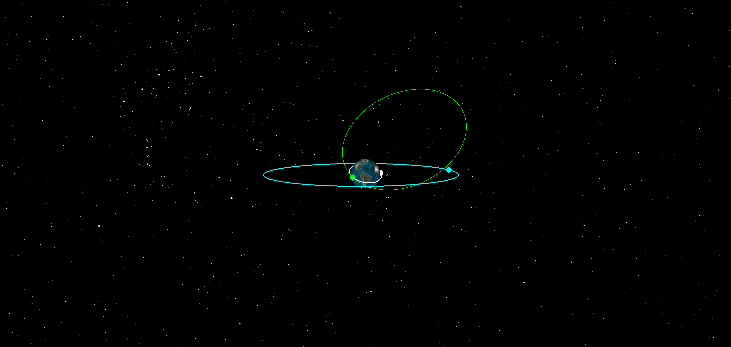
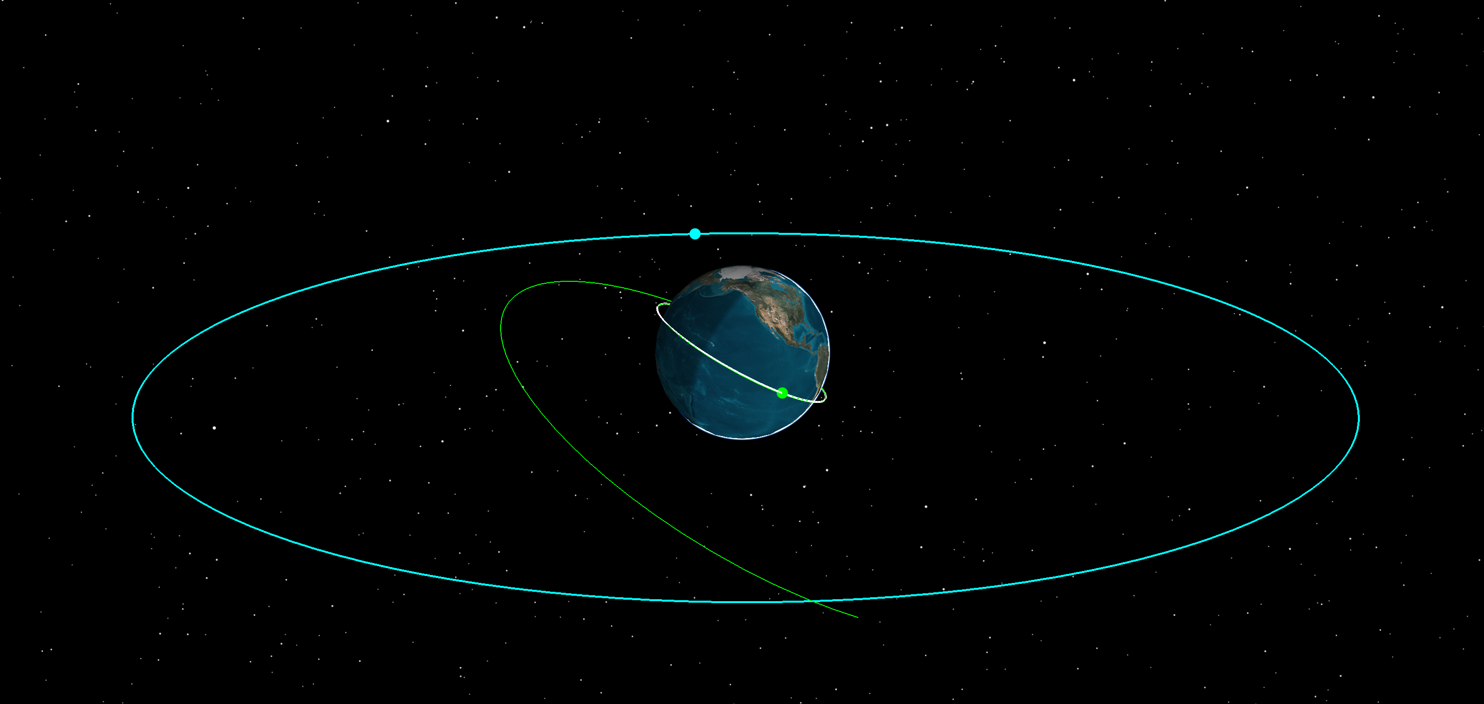
Transfer arc for the zero-revolution, long case
The long solution has increased the total Delta-V to approximately 23,500 m/sec, significantly more than the initial run.
One revolution: direction of motion is long and orbital energy is low
This is the first of the nonzero-revolution solutions to explore.
- Return to TransferBasic's () Properties ().
- Select Basic_Lambert () in the MCS.
- Open Lambert Profile's Properties () in the Profiles panel.
- Change the Number of Revolutions to 1.
- Make sure the Orbital Energy is set to Low.
- Leave the Direction of Motion as Long.
- Click .
- Click Run Entire Mission Control Sequence () in the MCS toolbar.
- Examine the 3D Graphics window.
- Refresh () the Maneuver Summary report and examine the total Delta-V.
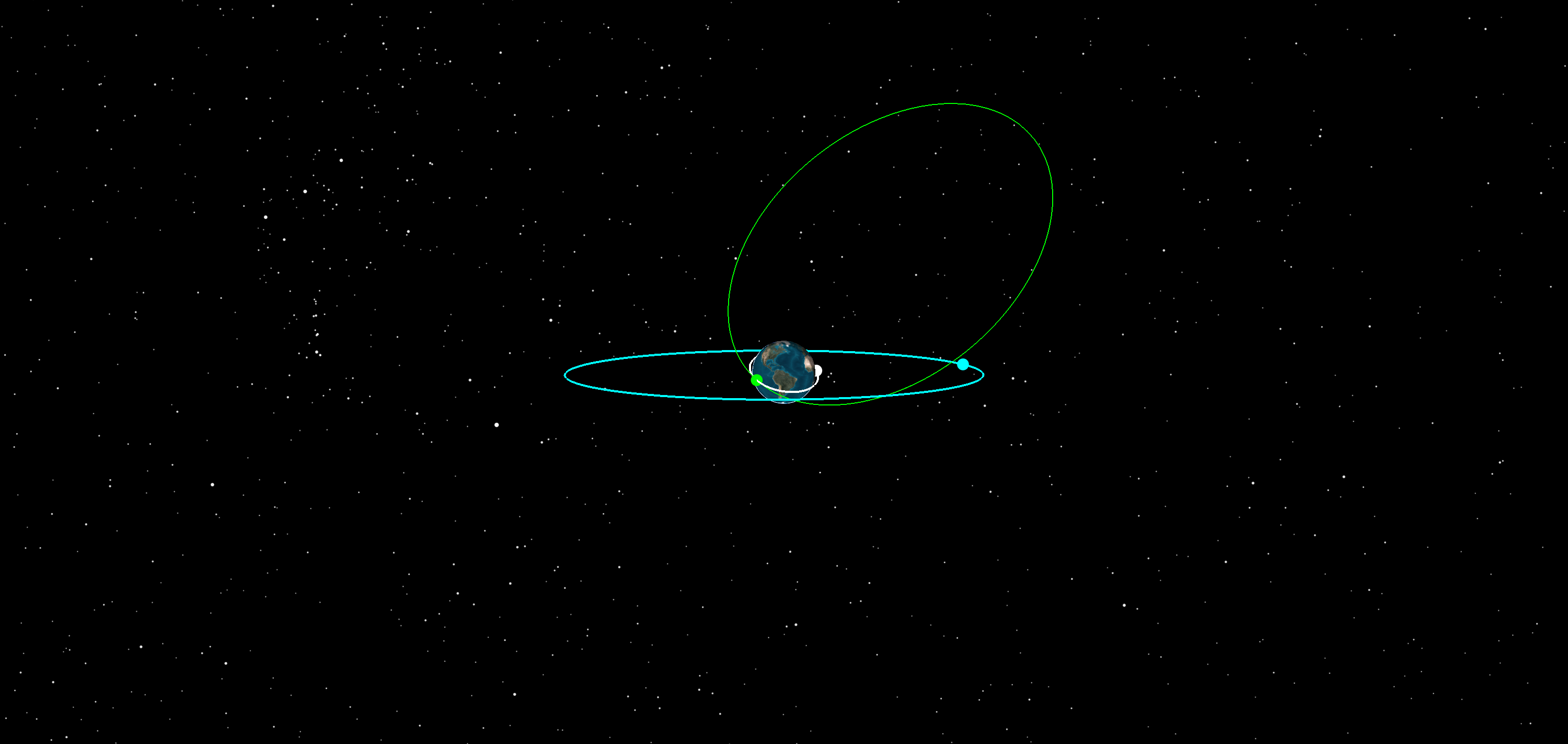
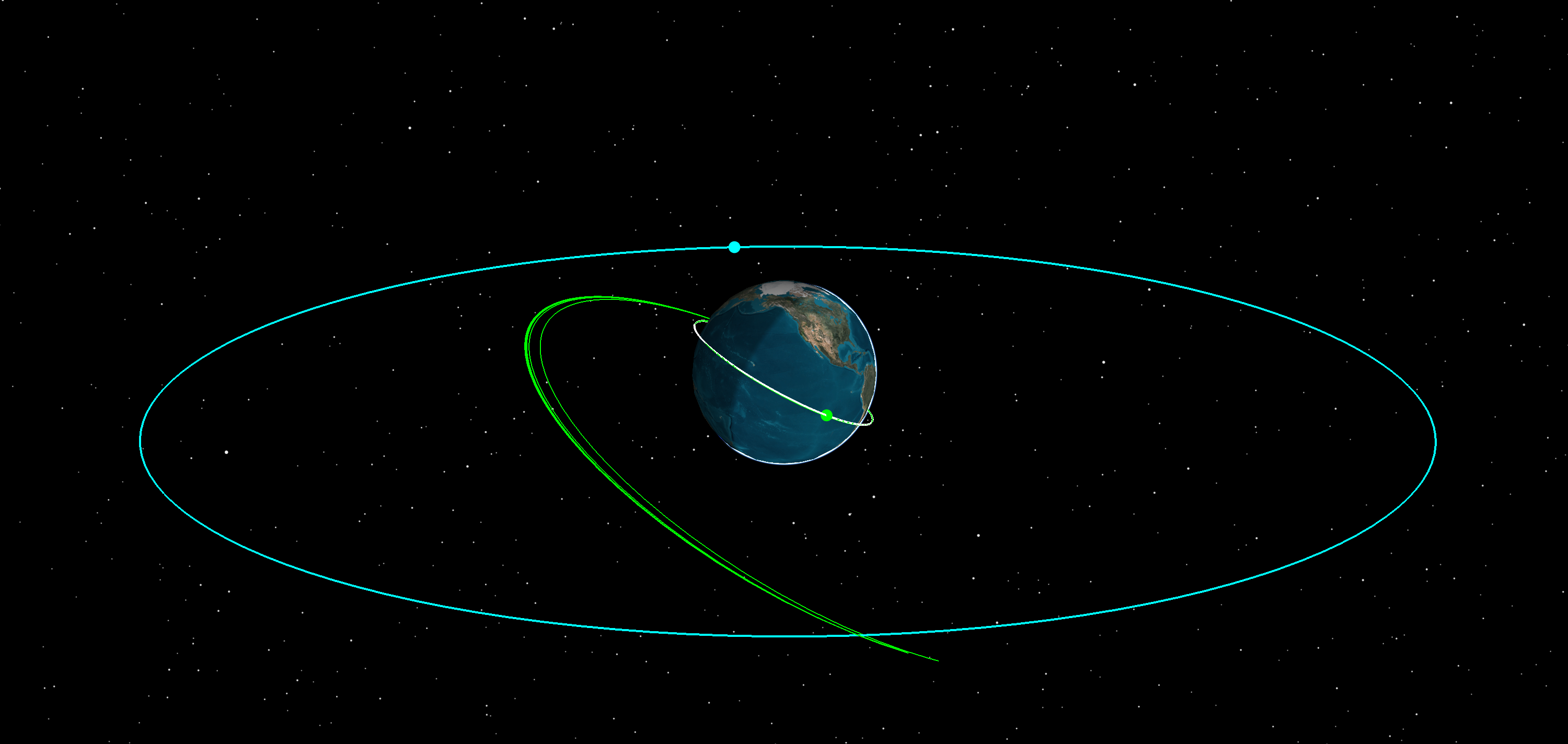
Transfer arc for the one-revolution, long, low case
The long solution has a total Delta-V of approximately 23,085 m/sec, about the same as the earlier long, zero-revolution solution.
One revolution: direction of motion is long and orbital energy is high
For this case, the number of revolutions stays at one, which enables you to change the orbital energy to high.
- Select Basic_Lambert () in the MCS.
- Open Lambert Profile's Properties () in the Profiles panel.
- Leave the Number of Revolutions as 1.
- Change the Orbital Energy to High.
- Leave the Direction of Motion as Long.
- Click .
- Click Run Entire Mission Control Sequence () in the MCS toolbar.
- Click for the Impact Warning.
- Examine the 3D Graphics window.
- Refresh () the Maneuver Summary report and examine the total Delta-V.
Transfer arc for the one-revolution, long, high case
This solution has a total Delta-V of approximately 23,095 m/sec. Unfortunately, it also causes the satellite to impact the Earth, which is obviously not acceptable.
One revolution: direction of motion is short and orbital energy is high
This time around, set the direction of motion to short and the orbital energy to high, and then examine the results.
- Select Basic_Lambert () in the MCS.
- Open Lambert Profile's Properties () in the Profiles panel.
- Leave the Number of Revolutions as 1.
- Leave the Orbital Energy as High.
- Change the Direction of Motion to Short.
- Click .
- Click Run Entire Mission Control Sequence () in the MCS toolbar.
- Examine the 3D Graphics window.
- Refresh () the Maneuver Summary report and examine the total Delta-V.
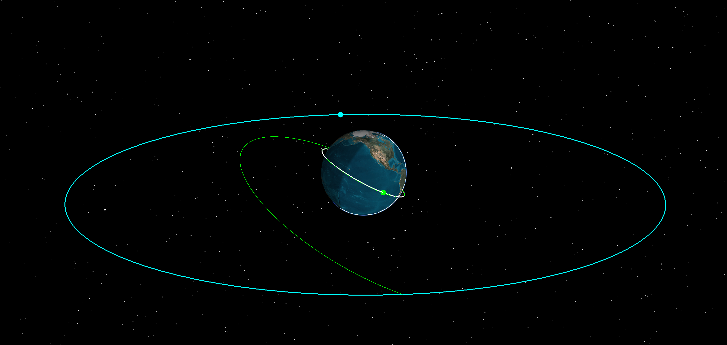
Transfer arc for the one-revolution, short, high case
This solution has decreased the total Delta-V to approximately 7,910 m/sec. While still impractical, this transfer has a lower Delta-V than your first solution!
One revolution: direction of motion is short and orbital energy is low
The final basic Lambert transfer arc involves setting the direction of motion to short and the orbital energy to low.
- Select Basic_Lambert () in the MCS.
- Open the Lambert Profile's Properties () in the Profiles panel.
- Leave the Number of Revolutions as 1.
- Change the Orbital Energy to Low.
- Leave the Direction of Motion as Short.
- Click .
- Click Run Entire Mission Control Sequence () in the MCS toolbar.
- Click for the Impact Warning.
- Examine the 3D Graphics window.
- Refresh () the Maneuver Summary report and examine the total Delta-V.
Transfer arc for the one-revolution, short, low case
Preparing for the next section
This solution has increased the total Delta-V to approximately 8,376 m/sec and it causes the satellite to impact the Earth. This is the final basic Lambert profile case, so close some items in preparation for the next part.
- Close the Maneuver Summary report and the Report & Graph Manager.
- Click to close TransferBasic's () Properties ().
Summarizing the Basic Lambert transfer
The combination of long direction of motion and high orbital energy and the combination of short direction of motion and low orbital energy both result in the transfer impacting the Earth, so they are unacceptable for these start, end, and time of flight conditions. Given the fixed time of flight of two days, the associated maneuver costs are substantially higher than typically employed. You would only consider these solutions if you had to meet specific geometry or timing requirements. Fortunately, there is a way to find better solutions.
Setting up the initial Lambert Search profile
The basic Lambert profile provided you with single solutions for given conditions. Now you will try the Lambert Search profile, which searches over many different solutions based on the conditions you set. For this profile, you will add a propagate sequence before the first maneuver. You will use this profile to find the minimum Delta-V for the mission of going from LEO to GEO.
Creating a new transfer satellite
Copy the TransferBasic satellite to create a new Satellite object.
- Select TransferBasic () in the Object Browser.
- Click Copy (
 ) in the Object Browser toolbar.
 - Click Paste().
- Rename TransferBasic1 () TransferSearch.
Creating a Lambert Search Target Sequence
Rename the existing Basic Lambert target sequence to a more appropriate name.
- Open TransferSearch's () Properties ().
- Select the Basic - Orbit page.
- Rename Basic Lambert () Search Lambert in the MCS.
Setting the segments in Search Lambert
Update the MCS segments for a Lambert Search profile.
- Drag the Propagate () segment to place it before Maneuver ().
- Right-click on Maneuver ().
- Select Insert After... in the shortcut menu.
- Select Propagate () in the Segment Selection dialog box.
- Click .
- Ensure the segment order is as shown:
TARGET SEQUENCE FOR A LAMBERT SEARCH
Changing the propagator
For the initial phase of the analysis, use a simple force model for the Propagate segments.
- Select Propagate () in the MCS.
- Check that Propagator (on the right) is set to Earth Point Mass.
- Select Propagate1 () in the MCS.
- Click the Propagator ellipsis ().
- Select Earth Point Mass ().
- Click .
Creating an initial Lambert Search profile
Create a new Lambert Search profile for the Search Lambert Target Sequence.
- Select Search Lambert () in the MCS.
- Click New... () in the Profiles panel on the right.
- Select Lambert Search Profile () in the New... dialog box.
- Click .
Changing the properties of the Lambert Search profile
Rather than looking for a transfer trajectory that has the satellite arrive in exactly two days, you will now look at trajectories that span at most one day and can depart from the initial LEO orbit after at most one day.
- Click Properties... () for the Lambert Search profile in the Profiles panel.
- Set the following:
- Click the Coordinate System ellipsis ().
- When the Select Reference dialog box opens, select GEO_Orbit () in the object list. This will cause the transfer to match the position of the GEO_Orbit satellite regardless of what the time of flight is.
- Select RIC (
 ) in the Systems for: GEO_Orbit list on the right.
 - Click to close the Select Reference dialog box.
- Click to close Lambert Search Profile's Properties .
| Parameter | Action |
|---|---|
| Latest Departure Time from Start of Target Sequence | Set this to 1 day. |
| Latest Arrival Time from the Start of Target Sequence | Set this to 1 day. |
| Grid Search Time Steps |
Set this to 200 seconds. Decreasing this value leads to a finer granularity solution search, which results in a solution closer to the true minimum. However computation time increases as a result. |
| Calculate Second Maneuver at Destination | Selected |
| Write Departure Delay to First Propagate | Select the check box and ensure that the segment below it is Propagate. |
| Write Initial Inertial Delta-V to Maneuver | Select the check box and ensure that the segment below it is Maneuver. |
| Write Flight Duration to Second Propagate | Select the check box and ensure that the segment below it is Propagate1. |
| Write Final Inertial Delta-V to Maneuver | Select the check box and ensure that the segment below it is Maneuver1. |
Calculating the Lambert Search transfer
Deactivate the basic Lambert profile and run your new Lambert Search profile for your MCS.
- Set the Mode for the (basic) Lambert Profile to Not Active.
- If created, set the Mode for the (basic) Lambert Profile1 to Not Active.
- Make sure that the Mode for the Lambert Search Profile is set to Active.
- Click Run Entire Mission Control Sequence () in the MCS toolbar.
- Clear the check box next to TransferBasic () in the Object Browser so that this arc does not appear in the graphics.
- Examine the 3D Graphics window.
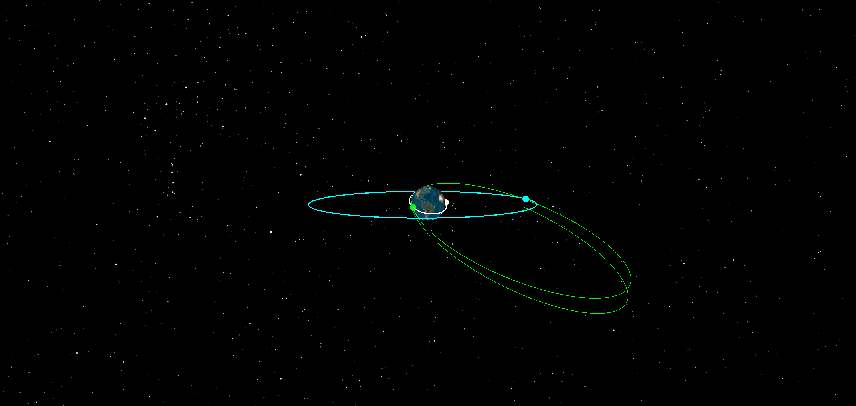
Initial Lambert Search profile transfer arc
The Lambert Search arc doesn't depart the starting orbit at the same place nor end at the same place as the prior arcs did. However, it does start and end on the same orbits as in the previous solutions. The difference in the starting orbit departure is due to the departure delay, and the difference in the ending position is because the GEO_Orbit satellite’s location in its orbit is consistent with the transfer time of flight.
Examining the results
View the results with a Maneuver Summary report.
- Right-click on TransferSearch () in the Object Browser.
- Select Report & Graph Manager ().
- Select the Maneuver Summary report in the My Favorites folder in the Styles panel.
- Click .
- Examine the total Delta-V in the report.
- Keep the report open for later use.
This solution has decreased the total Delta-V to approximately 4,100 m/sec. It is a good solution, but you should examine some additional parameter variations.
Refining the Lambert Search solutions
Examine the transfer angle next. It should be 180 degrees, or very close to 180 degrees, consistent with the known optimal two-impulse transfer solution, i.e., Hohmann. To get the transfer angle, subtract the mean anomaly at the arrival from the mean anomaly at departure, but recall that there is a propagation before the first maneuver. You need to find the time at the start of the first maneuver.
- Return to the Maneuver Summary report.
- Copy the Start Time of the first maneuver. It is an impulsive maneuver, so the start and stop times are the same.
Creating a mean anomaly report
Create a new custom report style to review the changes to the mean anomaly.
- Return to the Report & Graph Manager.
- Select the My Styles folder in the Styles panel.
- Click Create new report style () in the Styles toolbar.
- Name this report Mean_Anomaly and select the Enter key.
- On the left of the Report Style dialog box, expand () the Astrogator Values () data provider.
- Expand () the Keplerian Elems () data provider group.
- Select and move () the following data provider elements () to the Report Contents panel:
- Time
- MeanAnomaly
- Click to apply the changes and close the properties browser.
- Select the Mean_Anomaly report in the My Styles folder.
- Click .
Finding the mean anomaly value at Maneuver start
By looking through the Mean_Anomaly report you generated in the previous section, you can determine the mean anomaly at the start of the first maneuver.
- In the Interval section at the top of the page, click the selection arrow.
- Select Replace with Times.
- Paste the maneuver start time, copied from the Maneuver Summary report, into the Start Time field.
- Refresh () the report.
- Compare the mean anomaly at the start of the report with the final data entry of the report. The difference should be ~180 degrees, which is consistent with the known optimal two-impulse transfer solution.
Recall that the propagator used for this solution was the Earth Point Mass propagator. You can explore this solution further with higher-fidelity methods.
Switching to the full force solution for the Lambert Search
This is the first step in building a high-fidelity final solution. Modify the propagators to the full force model and run the MCS.
- Return to TransferSearch's () Properties ().
- Select Propagate () in the MCS.
- Click the Propagator ellipsis ().
- Select Earth Default High Fidelity v13 ().
- Click .
- Repeat steps 2-5 for Propagate1 ().
- Click Run Entire Mission Control Sequence () in the MCS toolbar.
- Select Search Lambert () in the MCS.
- Click under Profiles and Corrections. This creates LambertDuration stopping conditions in the propagate segments based on the results of the Lambert Search Profile and populates the Delta-V values of the maneuvers.
In the 3D Graphics window, you can see that the transfer orbit doesn't end in the proper orbit any more.
lambert search full force transfer arc
Setting up differential correction for the Lambert Search
By applying differential correction to the initial Lambert Search solution, you can gain more refined possibilities and hopefully save some fuel. Before diving into the differential corrector, you need to choose the control parameters and equality constraints to use with it. Follow the steps in the next five subsections to select parameters that become optional variables for the differential corrector.
Selecting the control parameters for the Propagate segment
Select the LambertDuration stopping condition as a control parameter for the Propagate segment.
- Select Propagate () in the MCS.
- Select LambertDuration in the Stopping Conditions panel on the right.
- Enable the Trip parameter as the independent variable by clicking the target icon () next to the Trip value box. You should see a white check mark appear over the icon.
Selecting the control parameters for the Maneuver segment
Next, select the Maneuver segment's Cartesian components as control parameters.
- Select Maneuver () in the MCS.
- Confirm that the radio dial for Cartesian is selected.
- Enable the X, Y, and Z Cartesian components as the independent variables by clicking the target icon () next to each. You should see a white check mark appear over each icon.
Selecting the control parameters for the Propagate1 segment
Set the Trip time as the control parameter for the Propagate1 segment.
- Select Propagate1 () in the MCS.
- Select the LambertDuration in the Stopping Conditions panel.
- Enable the Trip parameter as the independent variable by clicking the target icon () next to the Trip value box. You should see a white check mark appear over the icon.
Selecting the control parameters for the Maneuver1 segment
Select the Maneuver1 segment's Cartesian components as control parameters.
- Select Maneuver1 () in the MCS.
- Confirm that the radio dial for Cartesian is selected.
- Enable the X, Y, and Z Cartesian components as the independent variables by clicking the target icon () next to each. You should see a white check mark appear over each icon.
Setting the equality constraints
The equality constraint references a vehicle in the scenario, in this case the GEO_Orbit satellite. To set it:
- Go to the Basic - Reference property page of the TransferSearch satellite ().
- Select GEO_Orbit in the Reference Vehicle panel.
- Click . The GEO_Orbit satellite name should become bold.
- Return to the Basic - Orbit properties page of the TransferSearch satellite ().
- Select Maneuver1 () in the MCS.
- Click at the bottom of the MCS.
- When the User-Selected Results - Maneuver1 dialog box opens, expand () the Relative Motion () folder in the Available Components panel.
- Select and move () the following components ():
- CrossTrack
- CrossTrackRate
- InTrack
- InTrackRate
- Radial
- RadialRate
- Click to close the User-Selected Results - Maneuver1 dialog box.
- Click to accept your changes and keep the Properties window open.
Applying differential correction to Lambert Search
Now that you have chosen the variables for the differential corrector, you can begin solving for a higher-fidelity solution. Getting everything to converge in one differential corrector execution can be tricky, so split it up into three profiles. You will run these profiles individually, building on each other. The first profile (Best Timing) modifies the time of flight to get somewhat close to the final orbit. The second profile (Maneuver) modifies the first maneuver in order to match the correct position at the end of the transfer. The third profile (Maneuver1) modifies the second maneuver to match the correct velocity at the end of the transfer.
Setting up the best timing differential corrector
Create a new differential corrector and name it Best Timing.
- Select Search_Lambert () in the MCS.
- Click New... () in the Profiles toolbar on the right.
- Select Differential Corrector () in the New... dialog box.
- Click to close the New... dialog box.
- Rename Differential Corrector Best Timing in the Profiles panel.
- Click Properties... ().
- Select the Use check boxes for StoppingConditions.LambertDuration.TripValue for both the Propagate and Propagate1 objects in the Control Parameters panel.
- Select Use check boxes for the InTrack and Radial components in the Equality Constraints (Results) panel and set the Desired Values to 0.
- Click to close the Best Timing dialog box.
- Click to accept your changes and keep the Properties window open.
Computing the best timing
Run the entire MCS using the Best Timing differential corrector.
- Confirm that the Best Timing differential corrector's mode is set to Iterate.
- Set the mode for the Lambert Search Profile to Not Active.
- Ensure that Action is set to Run Active Profiles.
- Click Run Entire Mission Control Sequence () in the MCS toolbar.
- Click under Profiles and Corrections. This sets the transfer time.
- Examine the results in the 3D Graphics window. The transfer arc still does not end in the GEO orbit.
Lambert search transfer arc with best timing applied
Setting the initial maneuver differential corrector
This adjusts Maneuver to bring the satellite to the correct final position at the end of the transfer.
- Select Best Timing in the Profiles panel of Search Lambert's () Properties.
- Click Copy () and then Paste ().
- Rename Best Timing1 to Maneuver.
- With the Maneuver profile selected, click Properties ().
- In the Variable tab, under Control Parameters, confirm that the Use check boxes for StoppingConditions.LambertDuration.TripValue for both the Propagate and Propagate1 objects are still selected.
- Select the Use check boxes for the following Maneuver (not Maneuver1) control parameters:
- ImpulsiveMnvr.Pointing.Cartesian.X
- ImpulsiveMnvr.Pointing.Cartesian.Y
- ImpulsiveMnvr.Pointing.Cartesian.Z
- Select the Use check boxes for following components in the Equality Constraints (Results) panel and set the Desired Values to 0:
- CrossTrack
- Intrack
- Radial
- Set the tolerance to 0.001 km for the CrossTrack, InTrack, and Radial equality constraints.
- Click .
Computing the adjustment for Maneuver
Run the entire MCS for the Maneuver differential corrector.
- Confirm that the Maneuver differential corrector's mode is set to Iterate.
- Set all other profiles to Not Active.
- Click Run Entire Mission Control Sequence () in the MCS toolbar.
- Click under Profiles and Corrections. This sets the proper final position.
Setting the Copy of Maneuver differential corrector
Now that the satellite is at the correct ending position, this second maneuver gives the satellite the correct velocity at the end of the transfer.
- Return to Search Lambert () in the MCS.
- Right-click on the Maneuver profile in the Profiles panel and select Duplicate.
- Select the new Copy of Maneuver profile and click Properties ().
- Clear all the Use check boxes in the Control Parameters panel.
- Select the Use check box for the following Maneuver1 (not Maneuver) control parameters.
- ImpulsiveMnvr.Pointing.Cartesian.X
- ImpulsiveMnvr.Pointing.Cartesian.Y
- ImpulsiveMnvr.Pointing.Cartesian.Z
- Clear all the Use check boxes in the Equality Constraints (Results) panel.
- Select Use check boxes for the following equality constraints:
- CrossTrackRate
- IntrackRate
- RadialRate
- For each of the selected equality constraints, set the tolerance to 1e-06 km/sec.
- Click .
Computing the adjustment for Copy of Maneuver
Run the entire MCS for the Copy of Maneuver differential corrector.
- Confirm that the Copy of Maneuver differential corrector's mode is set to Iterate.
- Confirm that all other profiles are set to Not Active.
- Click Run Entire Mission Control Sequence () in the MCS toolbar.
- Click under Profiles and Corrections.
- Examine the 3D Graphics window and see that the transfer is now correct in the full force model.
- Refresh () the Maneuver Summary report and examine the total Delta-V.
This final search solution has a total Delta-V of approximately 4,100 m/sec.
Final Lambert search transfer arc
Comparing the Lambert Search solution to a Hohmann transfer
You can compare the final high-fidelity Lambert Search solution value with a Hohmann transfer. The Lambert Search transfer is a bit more complicated, modeling a transfer between an inclined LEO and GEO. The GEO in this tutorial is not perfectly circular, but for the moment assume for simplicity that the eccentricity of the GEO satellite is zero.
It will take a few steps to arrive at a final comparison fomula and value for the Hohmann transfer. The equations are from Wikipedia descriptions for
For the Hohmann transfer, the total Delta-V is the sum of the Delta-Vs for the first and second maneuvers:
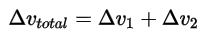
Delta-V for the first maneuver is:
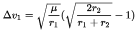
where:
- μ=GM is the standard gravitational parameter of the primary body, assuming M+m is not significantly bigger than M; for earth, this is μ ~ 3.986E14 m3 s−2.
- r1 is the initial orbital radius (7000000 m).
- r2 is the final orbit radius after the transfer (42000000 m).
Delta-V for the second maneuver is:
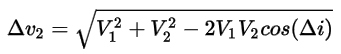
where Δi is the change in inclination.
V1 is the velocity of the transfer orbit at the end of the transfer (from the Vis-Viva Equation):
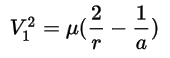
where
- r is the distance of the orbiting body from the primary focus. For r, use the target orbital radius (42000000 m).
- a is the semimajor axis of the body's orbit. For a, use the average of the target and source orbital radii (1/2 * (7000000 m + 42000000 m)).
V2 is defined as:

where r2 is the final orbit after the transfer.
Merging all those pieces, you find the equation for total Delta-V to be:
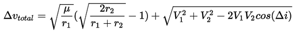
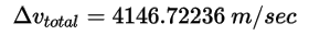
For the transfer between the inclined LEO and GEO in this tutorial, you'll find the Hohmann Transfer Delta-V to be 4,146.72236 m/sec. You could also model this Hohmann transfer in the STK application. This result is slightly higher than your Lambert Search high-fidelity solution, which was 4,100 m/sec. The Hohmann transfer is the optimal solution for circular orbits with no inclination change. Because the trajectories weren't simple orbit-raising maneuvers, the Lambert Search profile arrived at a more efficient Delta-V transfer solution.
Saving your work
- When finished, close any reports, graphs, and tools that are still open.
- Save () your work.
Summary
Exploring the solution space of transfers from LEO to GEO enables Engineers and Operators to optimize their mission. Using the Lambert Profile, you were able to examine the impact on Delta-V of long and short solutions with high and low energies. With the Lambert Search Profile, you were able to solve for first guesses for departure time, time of flight, and maneuver thrust vectors. This led to a fuel-efficient trajectory for the mission.
On your own
There are many settings that you did not use in this scenario, such as the Lambert Profile solution options (Minimum Eccentricity, Minimum Energy) and other Lambert Search Profile and differential correction solutions. Explore additional Lambert Profile and Lambert Search Profile options on your own.