STK Pro, STK Premium (Air), STK Premium (Space), or STK Enterprise
You can obtain the necessary licenses for this tutorial by
This tutorial requires STK 12.9 or newer to complete in its entirety. If you have an earlier version of STK, you can view a legacy version of this lesson.
The results of the tutorial may vary depending on the user settings and data enabled (online operations, terrain server, dynamic Earth data, etc.). It is acceptable to have different results.
Capabilities covered
This lesson covers the following capabilities of the Ansys Systems Tool Kit® (STK®) digital mission engineering software:
- STK Pro
- Communications
- Radar
Problem statement
Engineers and operators need a fast easy way to simulate radar systems for analysis. You need to determine how the following settings affect a radar's ability to track an aircraft:
- Aircraft radar cross section
- Pulse Repetition Frequency
- Antenna gain
- Pulse integration
- Clutter
Solution
Use the STK software's Radar capability to model an airport surveillance radar. You will:
- Build a monostatic radar.
- Test various settings against a test aircraft.
- Determine probability of detection.
If you are new to the STK application, review the following Level 1 - Beginner tutorials first: Part 1: Build Scenarios and Part 2: Objects and Properties.
What you will learn
Upon completion of this tutorial, you will understand:
- Radar cross sections
- Monostatic radars and their settings
- Radar data providers
Video guidance
Watch the following video. Then follow the steps below, which incorporate the systems and missions you work on (sample inputs provided).
Using the starter scenario (*.vdf file)
To speed things up and enable you to focus on this lesson's main goal, you will use a partially created scenario. The partially created scenario is saved as a visual data file (VDF) in your STK install.
Retrieving the starter scenario
- Launch the STK (
 ) application.
 - Click
 Open a Scenario in the Welcome to STK dialog box.
 - Go to <Install Dir>\Data\Resources\stktraining\VDFs.
- Select STK_Communications.vdf.
- Click .
Visual data files versus Scenario files
You must make sure that you save your work in the STK application as a scenario file (.sc) and not a visual data file (.vdf) by selecting Save As from the STK File menu. A VDF is a compressed version of an STK scenario, which makes them great for sending your work in the STK application to others. However, you should use a scenario file while working with the STK application on your machine.
If you open a VDF file, the STK application keeps it as a VDF and does not automatically convert it to a scenario file. This means that the STK application does not change the file type of your scenario when you launch your scenario. You need to convert the VDF to a Scenario file using Save As.
Saving a VDF file as a Scenario file
Use Save As from the STK File menu to convert the VDF file that you opened into a scenario file.
- Select Save As... in the File menu.
- Select the STK User folder in the navigation pane.
- Right-click in the file and folder browser.
- Select New > Folder in the shortcut menu.
- Rename New Folder to match the title of the scenario.
- Open the folder you just created.
- Enter the name of the folder into the File name field. This will be the Scenario object's name.
- Open the Save as type drop-down menu.
- Select Scenario Files (*.sc).
- Click .
Selecting relevant objects
In this lesson, you will analyze a radar's capability to track a test aircraft. You will only use a portion of the objects in the Object Browser, not all of them. There are extra objects because you can use this same scenario to complete other lessons about STKRadar and Communications.
- Select the check box for the following objects in the Object Browser:
- Radar_TestPlane (
 )
) - Radar_Site (
 )
) - Click Save (
 ). Save often during this lesson!
Specifying the radar cross section
Before setting up and constraining a radar system, the STK software's Radar capability enables you to specify an important property of a potential radar target — its radar cross section. Use the RCS of a popular single engine aircraft.
- Right-click on Radar_TestPlane () in the Object Browser.
- Select Properties (
 ).
). - Select the RF - Radar Cross Section page when the Properties Browser opens.
- Clear the Inherit check box at the top of the page.
- Set the Constant RCS Value to 10 dBsm (decibels referenced to a square meter).
- Click to accept your changes and to keep the Properties Browser open.
This enables you to set the RCS settings for the Aircraft (![]() ) object instead of inheriting the settings from the Scenario (
) object instead of inheriting the settings from the Scenario (![]() ) object.
) object.
Ideally, you would want to use an Aspect Dependent RCS file. Since you don't have one, you will use a constant value. The constant value you set is the RCS of a sphere that radiates isotropically.
Displaying radar cross section graphics
The 3D Graphics RCS page enables you to control the 3D display of Radar Cross Section contour lines.
- Select the 3D Graphics - Radar Cross Section page.
- Select Show Volume in the Volume Graphics panel.
- Select Show as wireframe.
- Enter 5 m in the Scale (Per dBsm) field.
- Click to accept your change and to close the Properties Browser.
Viewing the RCS in the 3D Graphics window
- Bring the 3D Graphics window to the front.
- Right-click on Radar_TestPlane () in the Object Browser.
- Select Zoom To.
- Use your mouse to zoom out until you can see the RCS sphere.
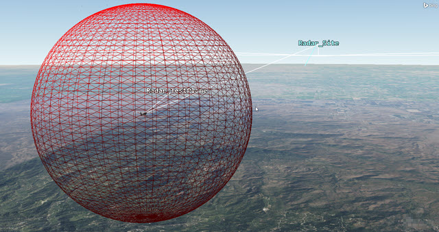
Radar Cross Section Sphere Surrounding the Test Plane
Inserting the antenna servo system
Insert a Sensor (![]() ) object to simulate a servo system for antenna positioning.
) object to simulate a servo system for antenna positioning.
- Zoom to Radar_Site () in the 3D Graphics window.
- Select Sensor (
 ) in the Insert STK Objects tool.
 - Select the Insert Default () method.
- Click .
- Select Radar_Site () in the Select Object dialog box.
- Click .
- Right-click on Sensor1 ().
- Select Rename in the shortcut menu.
- Rename Sensor1 () Servo_System.
Using a fixed antenna rather than a spinning antenna
In the STK application, you could create a spinning sensor to simulate a spinning radar antenna normally seen at an airfield. However in this scenario, you will lock the sensor onto the aircraft and constrain the sensor to point in a limited area. Not only is this ideal for testing, but it still simulates the actual field of view of the airfield surveillance radar both horizontally and vertically.
Defining the sensor field of view
Define Servo_System's (![]() ) field of view using a simple conic sensor pattern. You will use the sensor's field of view for situational awareness when Servo_System (
) field of view using a simple conic sensor pattern. You will use the sensor's field of view for situational awareness when Servo_System (![]() ) points the antenna at the target.
) points the antenna at the target.
- Open Servo_System's () Properties ().
- Select the Basic - Definition page.
- Enter 3 deg in the Cone Half Angle field.
- Click .
Where exactly is the Sensor object by default?
When you attach the Sensor (![]() ) object to the Place (
) object to the Place (![]() ) object, the sensor attaches to the Place object's center point. That center point is on the surface of local terrain, but you want your servo system 50 feet above the terrain. You can move location of the sensor in relation to the Place object by increasing the sensor's fixed displacement vector. Later, when you attach the Radar (
) object, the sensor attaches to the Place object's center point. That center point is on the surface of local terrain, but you want your servo system 50 feet above the terrain. You can move location of the sensor in relation to the Place object by increasing the sensor's fixed displacement vector. Later, when you attach the Radar (![]() ) object to the Sensor (
) object to the Sensor (![]() ) object , the radar's antenna will also be 50 feet above the terrain.
) object , the radar's antenna will also be 50 feet above the terrain.
Increasing the height of the sensor
Set the sensor 50 ft off of the ground using the fixed displacement vector found in the Sensor object's Properties.
- Select the Basic - Location page in Servo_System's () Properties ().
- Open the Location Type drop-down menu.
- Select Fixed.
- Enter -50 ft in the Z field.
- Click .
The Place object's positive Z points to Earth's center. Therefore, to raise Servo_System (![]() ) above the ground, you use a negative value.
) above the ground, you use a negative value.
Targeting the Aircraft object with the Sensor object
Use the Targeted pointing type to point Servo_System (![]() ) at Radar_TestPlane (
) at Radar_TestPlane (![]() ).
).
- Select the Basic - Pointing page in Servo_System's () Properties ().
- Open the Pointing Type drop-down menu.
- Select Targeted.
- Move (
 ) Radar_TestPlane () from the Available Targets list to the Assigned Targets list.
 - Click .
Setting range and elevation angle constraints
Typically, an airport surveillance radar has a nominal range of 60 miles and has a beam with an the elevation angle of 30 degrees. This means the radar can track the aircraft while flying within 60 miles at an angle between 0 and 30 degrees. Anything flight higher than 30 degrees is the "cone of silence" where the radar cannot track the aircraft.
- Select the Constraints - Active page.
- Click Add new constraints (
 ) in the Active Constraints toolbar.
 - Select Elevation Angle in the Constraint Name list in the Select Constraints to Add dialog box.
- Click .
- Click to close the Select Constraints to Add dialog box.
- Select the Max: check box in the Elevation Angle panel in the Constraint Properties section
- Enter 30 deg in the Max field.
- Click to accept your changes and to close the Properties Browser.
Inserting an airport surveillance radar to the sensor
Insert a Radar (![]() ) object to create an airport surveillance radar. You will model some airport surveillance radar specifications that are easily available to the public.
) object to create an airport surveillance radar. You will model some airport surveillance radar specifications that are easily available to the public.
Inserting a radar object
First, insert a Radar (![]() ) object.
) object.
- Insert a Radar (
 ) object using the Insert Default () method.
 - Select Servo_System () in the Select Object dialog box.
- Click .
- Rename Radar1 () ASR.
Modeling a monostatic radar
You will model a monostatic radar using a search track mode. You could use this type of antenna for transmitting and receiving, along with detecting and tracking point targets.
To understand constants and equations used in the STK application, look at Search/Track Radar Constants and Equations in STK Help.
- Open ASR's () Properties ().
- Select the Basic - Definition page.
- Notice how the Radar System defaults to Monostatic.
- Select the Mode tab.
- Notice how the Radar Monostatic Mode defaults to Search Track.
Defining the waveform
The waveform in your system will use a fixed pulse repetition frequency (PRF) of approximately 1000 Hz. Radar systems often use multiple pulse integration which is the process of summing all the radar pulses to improve detection. This helps increase the signal-to-noise ratio. The PRF is the number of pulses of a repeating signal in a specific time unit. After producing a brief transmission pulse, the transmitter turns off in order for the receiver to hear the reflections of that signal off of targets.
- Select the Pulse Definition subtab.
- Notice the Waveform is set to Fixed PRF.
- Notice the default PRF value is 0.001 MHz.
You will keep that value since your system's PRF is approximately 1000 Hz.
Defining the pulse width
Pulse width is the width of the transmitted pulse. The uncompressed RF bandwidth can also be taken as the inverse of the pulse width. You will set the pulse width to one microsecond.
- Open the Pulse Width unit selector (
 ).
). - Select usec.
- Set the Pulse Width to 1 usec in the Pulse Width field.
- Click .
Defining the antenna pattern
Model the antenna using the cosine squared aperture rectangular antenna pattern. The antenna transmit frequency for your radar is between 2.7-2.9 GHz.
- Select the Antenna tab.
- Click the Antenna Model Component Selector (
 ).
). - Select Cosine Squared Aperture Rectangular (
 ) in the Antenna Models list when the Select Component dialog box opens.
 - Click to accept your selection and to close the Select Component dialog box.
- Select the Use Beamwidth option.
- Set the following:
- Click .
| Option | Value |
|---|---|
| X Dim Beamwidth | 5 deg |
| Y Dim Beamwidth | 1.4 deg |
| Design Frequency | 2.8 GHz |
| Main-lobe Gain | 34 dB |
| Efficiency | 55% |
Defining the radar transmitter
The transmitter has a frequency range of 2.7-2.9 GHz, a peak power of 20 kilowatts, and uses either linear or circular polarization. Your system uses linear polarization.
- Select the Transmitter tab.
- Select the Specs tab.
- Select the Frequency option.
- Enter 2.8 GHz in the Frequency field.
- Enter 20 kW in the Power field.
- Select the Polarization subtab.
- Select the Use check box.
- Keep the default setting of Linear.
- Click .
Setting the radar receiver's polarization
You don't have specific values regarding the low noise amplifier settings. These would be applied on the Receiver's Specs subtab. However, you know the polarization.
- Select the Receiver tab.
- Select the Polarization subtab.
- Select the Use check box.
- Ensure the default setting is Linear.
- Click .
Defining radar clutter
Radar clutter is unwanted echoes returning to your radar system. Such echoes typically result from ground, sea, rain, animals, insects, chaff, and atmospheric turbulence. Your radar site is surrounded by buildings, hills, and mountains. You want to take this into account during your analysis.
- Select the Clutter tab.
- Select the Enabled check box.
Scattering Point Provider List
The STK software defaults to one scattering point provider list and defaults to one provider (single point). You can build your own lists and save them to the Component Provider. You can choose a Scattering Point Provider that specifies the geometry needed for your calculations. For your preliminary analysis, you will use a nominal points file. A points file is an ASCII text file that needs to have a *.spf extension.
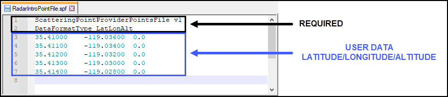
Points File
Creating a points file
Create a points file and save it in your scenario folder.
- Open Notepad or a text editor that does not add any hidden characters.
- Enter manually or copy and paste the following into Notepad:
- Open the File menu.
- Select Save As... .
- Browse to your scenario folder (e.g., C:\Users\<username>\Documents\STK_ODTK 13\<Scenario folder>).
- Open the Save as type drop-down list.
- Select All Files.
- Enter RadarPointFile.spf in the File name field.
- Click .
- Close Notepad.
ScatteringPointProviderPointsFile v1
DataFormatType LatLonAlt
35.41000	-119.03600	0.0
35.41100	-119.03400	0.0
35.41200	-119.03200	0.0
35.41300	-119.03000	0.0
35.41400	-119.02800	0.0
Configuring the Scatter Point Model
- Click the Scattering Point Provider Component Selector () in the Point Provider Details panel.
- Select Points File () in the Scattering Point Provider list when the Select Component dialog box opens.
- Click to accept your selection and to close the Select Component dialog box.
- Click the Filename ellipsis ().
- Browse to your scenario folder (e.g., C:\Users\<username>\Documents\STK_ODTK 13.1.0\<Scenario folder>).
- Select RadarPointsFile.spf.
- Click .
- Click .
When you select a points file, the STK software defaults to a constant coefficient of 0 dB. You can create your own component and change the value at any time. You can manually enter the value here which is then applied to all of your points. You will learn more about this later.
Computing access between the radar and the aircraft
You want to create an Access report between the radar and the aircraft to better analyze your radar system. The Access report will show you the exact times when the radar system can track the aircraft. Also the report will visualize those times on the 2D and 3D Graphics windows using access lines.
Modifying the radar graphics options
The Access page of ASR's 2D Graphics properties enables you to control the display of radar access lines in the 2D Graphics window. It also enables you to see the points from your points file in both the 2D and 3D Graphics windows.
- Select the 2D Graphics - Access page.
- Select the Enable check box in the Clutter panel.
- Open the Color drop-down menu.
- Select yellow.
- Click to accept your changes and to close the Object Browser.
Creating the Access report
You will create the Access report.
- Right-click on ASR () in the Object Browser.
- Select Access... (
 ) in the shortcut menu.
 - Select Radar_TestPlane () in the associated objects list once the Access Tool opens.
- Click
 .
. - Leave the Access Tool open.
Visualizing your points from the points file
After creating an access between the radar and the aircraft, you can visualize the points from the points file in both the 2D and 3D Graphics windows.
- Bring the 3D Graphics window to the front.
- Zoom to Radar_Site ().
- Use your mouse to zoom out until you can see all five points from the points file.
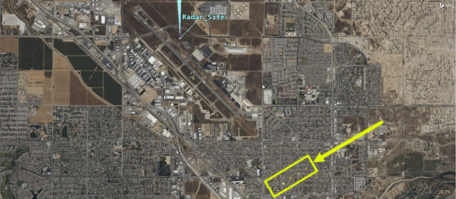
Point File Points 3D Graphics Window
Creating a custom report
You will create a custom report to draw specific data from your scenario, enabling you to tailor your analysis to your needs. This custom report will gather a lot of information like the Signal to Noise Ratio (SNR), Probability of Detection (PDet), pulse integration, and clutter.
Creating a new report
First create a new report.
- Return to the Access Tool.
- Click .
- Select the My Styles (
 ) folder in the Styles panel list once the Report & Graph Manager opens.
 - Click Create new report style (
 ) in the Styles toolbar.
 - Name the report Radar Test.
- Select the to open the report's properties.
- Select the Content page when the Properties Browser opens.
Selecting your data providers
Data providers let you decide what information you want the report to gather. For this scenario, you will base the probability of detection (PDet) on a value of 0.800000 or higher (with 1.0 being the highest value). You will want information like the signal-to-noise ratio, pulse integration, and clutter.
- Expand (
 ) the Radar SearchTrack (
 ) data provider in the Data Providers list.
 - Move () the following data provider elements, in the order shown, to the Report Contents list:
- Time (
 )
) - S/T Integrated SNR (): Signal to Noise ratio over the dwell of pulses for the primary polarization channel
- S/T Integrated S/(N+J+C) (): Signal to Noise plus Jamming plus Clutter ratio over the dwell of pulses under jamming presence for the primary polarization channel
- S/T Integrated PDet (): Probability of Detection integrated over the dwell of pulses for the primary polarization channel
- S/T Integrated PDet w/J+C (): Probability of Detection under jamming and clutter presence for the primary polarization channel
- S/T Clutter Power (): Clutter power for the primary polarization signal channel
- S/T Pulses Integrated (): Number of pulses
- Click .
Generating your report
- Select Radar Test (
 ) in the My Styles () folder when you return to the Report & Graph Manager.
 - Click
- Focus on the first access when the report opens.
- Scroll down in the report to when Time equals approximately 18 minutes.
- Scroll down in the report until Time equals approximately 30 minutes.
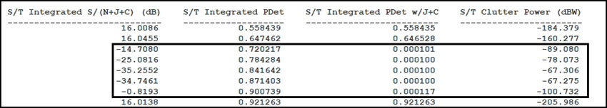
- Look at your S/T Integrated PDet value at 1 Aug 2022 19:22:42.00.
You require an S/T Integrated PDet of 0.800000 or better. The first S/T Integrated PDet value in the report is bad. You can also see that S/T Pulses Integrated is 512, which is the maximum default number set in the Radar (![]() ) objects properties.
) objects properties.
S/T Integrated PDet jumps above 0.800000. You can see a corresponding decrease in S/T Pulses Integrated.
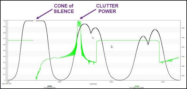
You can see about a three-minute break between the first group of accesses. Then, the accesses resume. The aircraft flew through the radar's cone of silence.
Analyzing your custom graph
The value at 1 Aug 2022 19:22:42.00 is above 0.800000. However, the next column to the right (S/T Integrated PDet w/J+C) the value is 0.000100, which is very low. From this data, you can determine that clutter is degrading your system. You can see the clutter increase in the next column, S/T Clutter Power (dBW). As the clutter power increases, your S/T Integrated PDet values decrease. You can also see that S/T Integrated S/(N+J+C) (dB) (SNR) is greatly affected by increased S/T Clutter Power (dBW).
Clutter Effect
Creating a custom graph
Creating a graph can make trends in your data easier to analyze and improves your briefings or presentations. For this graph, you will focus on Probability of Detection and Clutter Power.
Creating a new graph
First create a new graph.
- Close the Radar Test report.
- Return to the Report & Graph manager.
- Select the My Styles () folder in the Styles panel.
- Click Create new graph style (
 ) in the Styles toolbar.
 - Name the graph PDET and Clutter Power.
- Select the Enter key.
- Select the Content page when the Properties Browser opens.
Selecting your data providers
You will graph S/T Integrated PDet and S/T Clutter Power.
- Expand () the Radar SearchTrack () data provider in the Data Providers list.
- Move () S/T Integrated PDet () data provider element to the Y Axis.
- Move () S/T Clutter Power () data provider element to the Y2 Axis.
- Enter 1.000 sec in the Step Size field.
- Click .
Generating your custom graph
- Return to the Report & Graph Manager.
- Select PDET and Clutter Power (
 ) in the My Styles () folder.
 - Click .
Be patient. This can take a couple of minutes to analyze.
Analyzing your custom graph
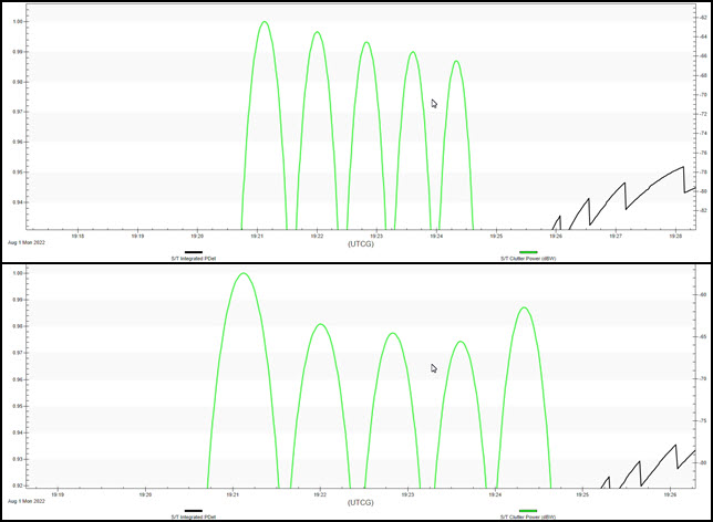
There are two areas of interest in the graph. First, you can see a break during the first period of tracking the aircraft. This is the aircraft passing through the radar's cone of silence. During the second period of tracking, you can see where clutter effects your PDET.
PDET and Clutter Power Graph
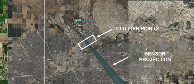
Viewing clutter in the 3D Graphics window
You can see that your points file works in the both the 2D and 3D Graphic windows.
- Place your cursor in the middle of the clutter spike in the PDET and Clutter Power graph.
- Right-click.
- Select Set Animation Time in the shortcut menu.
- Bring the 3D Graphics window to the front.
- Zoom out until you can see Servo_System's () projection passing through the clutter points.
- Return to the PDET and Clutter Power graph.
- Hold down your left mouse button, draw a box around the clutter spikes and zoom into the top of the clutter spikes. You can see each individual point's power spike.
- Keep the PDET and Clutter Power graph open.
Sensor and Clutter Points
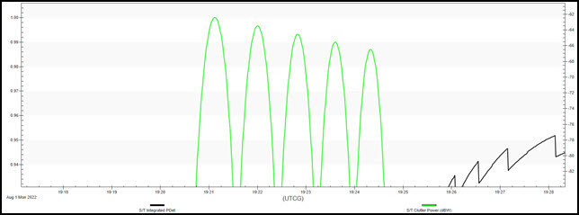
Point Power Spikes
Creating a constant coefficient component
Recall that the constant coefficient applied to all of the points in your file is 0 dB. Some points in the file might have larger values. You can create your own component and apply different coefficient values to different points.
- Open ASR's () properties ().
- Select the Basic - Definition page when the Properties Browser opens.
- Select the Clutter tab.
- Click the Scattering Point Model Component Browser (
 ) in the Default Scattering Point Model panel.
Duplicating a component
The components in the Scattering Point Model list cannot be changed. However, you can duplicate a component and then edit the duplication.
- Select Constant Coefficient () in the Scattering Point Model list.
- Click Duplicate component (
 ) in the Scattering Point Model toolbar.
 - Type My Coefficient in the Name: field when the Field Editor dialog box opens.
- Click to close the Field Editor dialog box.
- Double-click on My Coefficient (
 ) in the Scattering Point Model list.
 - Enter 5 dB in the Constant Coefficient field when the ScatteringPointModel - My Coefficient dialog box opens.
- Click to close the ScatteringPointModel - My Coefficient dialog box.
- Click to close the Component Browser.
Navigating to the points file
You can select individual points in your points file to use your custom coefficient component.
- Open Windows File Explorer.
- Select Documents when File Explorer opens.
- Double-click on STK_ODTK 13 ().
- Double-click on your scenario folder ().
- Right-click on RadarPointFile.spf.
- Select Open with.
- Select Notepad in the dialog box.
- Click .
Editing the points file
- When Notepad opens, enter "My Coefficient" (include the double quotation marks) to the right of the first point. You have to enter the exact name of the component you created.
- Enter "My Coefficient" to the right of the last point.
- Open the File menu.
- Select Save.
- Close Notepad and File Explorer.
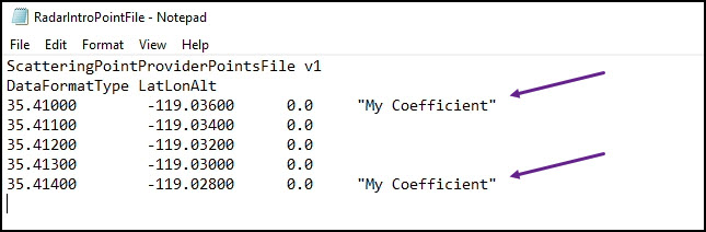
Edited Points File
Reloading your points file
You must reload your points file in order for the changes to take effect.
- Return to ASR's () properties.
- Click in the Point Provider Details panel. You should see change in the points list in the ScatteringPointModel column.
- Click .
Be patient. This can take a couple of minutes to analyze.
Viewing the changes in the PDET and Clutter Power graph
- Return to the PDET and Clutter Power graph.
- Click Refresh (
 ) in the report tool bar or select the F5 key to refresh.
 - Zoom into the top of the clutter spike to see changes.
Coefficient Comparison
The first graph shows a constant coefficient of 0 dB on all five points. The second graph shows a 5 dB increase for the first and last points.
Saving your work
- Close any open reports, tools, and properties.
- Save () your work.
Summary
You created a scenario that used the surface of the WGS84 as the central body obstruction. You entered a constant RCS value for your aircraft. You built a servo system to track your aircraft. You set up an airport surveillance radar using a monostatic search track mode. Then, you learned how to measure clutter effects using a points file. You learned about data providers required to analyze your radar system. Lastly, you created a custom component which increased the constant coefficient and applied the component to two points in the points file.