The Ansys RF Channel Modeler™ plugin is installed separately from the base installation of the Ansys Systems Tool Kit® (STK®) digital mission engineering software. If you wish to evaluate the capability, you may download just the plugin or the full install
Pictures, graphs, and data snippets are used as examples only. The results of the tutorial may vary depending on the user settings and data enabled (online operations, dynamic Earth data, etc.). It is acceptable to have different results.
Capabilities covered
This lesson covers the following capabilities of the Ansys Systems Tool Kit® (STK®) digital mission engineering software:
- STK Communications and Radar (especially the RF Channel Modeler plugin)
Problem statement
You want to create a radar image of a scene, which contains a parked aircraft, from a low-flying aircraft that is passing by the scene. You have to account for antenna capability, angular velocity, and signal reflections. You want to see how how well the aircraft radar can image the scene, which contains buildings, trees, and special object. You can then make a movie of the sampled images of the scene as the aircraft flies by. This exercise gives you the basic capability to then launch your own further study of varying aspects such as aircraft flight path, target placement, antenna parameters, radar imaging parameters, etc. The cost is high if you try this using real equipment in real scenes, so you need to simulate this instead.
Solution
You can use the STK software to model all the objects, facets, and antenna placements in your analysis. You can then employ the RF Channel Modeler plugin inside of the STK application to design analysis configurations that include analysis extents, antenna types, waveform settings, transceivers, targets, scene contributors, and radar image data product settings. Running an analysis configuration produces an HDF5 file that contains high-fidelity scattering parameter antenna-to-antenna coupling data for all of your analysis configurations. By looking at plots of the data, you can determine the performance of your radar imaging.
Ultimately, you could enhance this exercise to fly your aircraft along different routes and run more RF Channel Modeler analysis configurations with and without the scene facet tileset data. This would help you to find the optimum imaging flight path for the mission. For this tutorial, you will just look at one flight path.
For more information on setting up analysis configurations, see the RF Channel Modeler Help.
You can run the RF Channel Modeler plugin through the RFCM API. For a description of available sample code, see the RF Channel Modeler section of the Plugin Samples topic page in the STK Programming Help. If you execute the RF Channel Modeler plugin through the Object Model, you must set the following system environment variables:
ANSYSCL252_DIR: Set this to the licensing client directory in your install directory at <Install Dir>\licensingclient.
ANSYSLIC_DIR: Set this to the licensing folder located in your install directory at <Install Dir>\Shared Files\Licensing.
What you will learn
Upon completion of this tutorial, you will be able to:
- Create a basic STK scenario for radar detection and radar imaging.
- Load in a facets tileset.
- Set up RF Channel Modeler analysis configurations for radar, including the specification of analysis extents, antenna types, waveform settings, transceivers, targets, and imaging product data settings.
- Produce plots of the results of the RF Channel Modeler radar analysis runs and see radar images for your analysis setup.
Learning the STK application
If you are new to the STK application, consider first walking through the following Level 1 STK tutorials to become familiar with the basic functionality needed for setting up scenarios for the RF Channel Modeler plugin.
Level 1, Part 1: Build Scenarios
Level 1, Part 2: Objects and Properties
Verifying the RF Channel Modeler plugin is installed
Ensure that the RF Channel Modeler plugin is installed on your computer.
- Open the STK application (
 ). In the initial dialog box, the RF Channel Modeler plugin should be in the list under "Additional Capabilities."
 - Select the check box next to "RF Channel Modeler" before continuing. Doing so ensures that the plugin is available within the STK application.
See the next section for how to proceed in the STK application.
Creating a new scenario
You must create an STK scenario. Then you can set up your RF Channel Modeler analyses. You already launched the STK application and should now see the Welcome to STK dialog box.
- Click
 Create a Scenario.
 - Enter "RFCM_Radar" as the Name in the STK: New Scenario Wizard and leave everything else as the default values.
- Click when you finish.
- Click Save (
 ) after the scenario loads. The STK application creates a folder with the same name as your scenario.
 - Verify the scenario name and location in the Save As dialog box.
- Click .
Save (![]() ) the scenario after each section of this tutorial!
) the scenario after each section of this tutorial!
Enabling your GPU in STK
To run an RF Channel Modeler analysis, you need to let the STK application know the Graphics Processing Units (GPUs) that you have available on your computer to use. You must have at least one available and registered in the STK application.
- Go to the Edit menu in the STK application and select Preferences.
- Go to the RF Channel Modeler page.
- Make sure at least one Enabled check box is selected next to an available GPU on the GPU Properties pane.
- Click to accept any changes and close the Preferences dialog box.
Setting up the scenario
You will want to use epoch seconds as the time units for your scenario, since you want to generate results that start at time 0.0 seconds. This makes it easier for selecting times to view plots.
- Double-click the RFCM_Radar scenario object in the Object Browser to bring up its Properties Browser.
- Go to the Basic - Units page.
- Select DateFormat under Dimension.
- Under Current Unit, click the box next to DateFormat.
- Use the drop-down menu to select Epoch Seconds (EpSec) as the units.
- Click to save this change and close the Properties Browser.
- Close the 2D Graphics window. You will not need this.
- Click the deletion "X" near the bottom of the STK application UI to delete the Timeline View section. You will not need this either, and deleting it creates more room for viewing the RF Channel Modeler plugin UI later.
Adding a facets tileset to the STK application
You need to add a facets tileset to the STK application that at least covers the area of your analyses. This tileset provides 3D modeling of known stationary structures and terrain in the covered area.
- Go to the 3D Graphics window.
- Click the Globe manager icon (
 ) in the toolbar.
 - Make sure you are in the Hierarchy tab in the Globe Manager window.
- Click the Add Terrain/Imagery icon (
 ).
). - Select Add 3D Tilesets.
- Select the check box next to the AGI_Headquarters tileset.
- Click .
- Click in the Use Tileset for Analysis dialog box.
- Close the Globe Manager window.
Creating a Place object
Create a Place object that you can designate as the focal point of your radar image. For this tutorial, you will assign the Place object to a location approximately in the middle of the courtyard of the three buildings. In the 3D Graphics window, the Place object will look like a 10 cm sphere.
- Click the Insert Object icon (
 ).
). - Select Place (
 ) on the left and Define Properties (
 ) on the right.
 - Click . You should see the Basic - Position page of the Place1 properties.
- Change the following property values:
Property Value Latitude 40.039 deg Longitude -75.5968 deg Height Above Ground 0.005 km - Select the Use terrain data check box, if not already selected.
- Go to the 3D Graphics - Model page.
- Select the Show check box in the Model pane.
- Click the ellipsis (
 ) next to Model File and browse to and select the Quad_Sphere_10cm.glb file in your install folder at <Install Dir>\Data\Resources\stktraining\samples. This is a 10 cm sphere model.
 - Click to apply and close the properties.
- Click Place1 in the STK Object Browser, right-click, and select Zoom To. Zoom out a little to bring in the surrounding scene. In the 3D Graphics window, you can see that Place1 is about in the middle of the courtyard, 5 m above the terrain. Of course, the sphere is very small relative to the scene items. If you want to move the center of your radar image, you can simply adjust the position of this sphere.
Inserting an Aircraft object
For your analysis, you will want to have a radar transceiver. Create an Aircraft object to anchor the location of the radar transceiver.
- Click the Insert Object icon ().
- Select Aircraft (
 ) on the left and Define Properties () on the right.
 - Click . You should see the Basic - Route page of the Aircraft1 properties.
Creating waypoints and a model for the aircraft
You will set up Aircraft1 (![]() ) so that it will fly by the three main buildings in your tileset such that it can see into the courtyard area surrounded by three buildings. You do not need to set Accel, Time, or Turn Radius; just accept the default values for these.
) so that it will fly by the three main buildings in your tileset such that it can see into the courtyard area surrounded by three buildings. You do not need to set Accel, Time, or Turn Radius; just accept the default values for these.
- Click on the Basic - Route page of Aircraft1's properties.
- Set the following for the first waypoint:
- Click .
- Set the following for the second waypoint:
- Set Reference to Terrain and Interp Method to Terrain Height in the Altitude Reference section of the page.
- Go to the 3D Graphics - Model page.
- Select the Show check box in the Model pane.
- Near the top, click the ellipsis () next to Model File.
- Select the helicopter file and click .
- Click to accept all changes and close the Aircraft1 Properties Browser.
| Option | Value |
|---|---|
| Latitude | 40.026 deg |
| Longitude | -75.57 deg |
| Altitude | 0.500000 km |
| Speed | 0.0463 km/sec |
| Option | Value |
|---|---|
| Latitude | 40.06 deg |
| Longitude | -75.60 deg |
| Altitude | 0.5000000 km |
| Speed | 0.0463 km/sec |
You now have a helicopter flying at 500 m altitude while passing close to the scene you want to image.
Inserting a Sensor object for Aircraft1
Add a sensor and attach it to Aircraft1. You must have a Sensor object in your STK scenario as the host for any transceiver in the RF Channel Modeler plugin.
- Click the Insert Object icon ().
- Select to insert a Sensor (
 ) object using the Define Properties () method.
 - Click .
- Attach the sensor to Aircraft1 in the Select Object dialog box.
- Click . The Basic - Definition page of the Sensor1 properties should appear.
- Set Cone Half Angle to 5 degrees.
- Go to the Basic - Pointing page.
- Set Pointing Type to Targeted.
- Select Place1 under Available Targets and move (
 ) it to the Assigned Targets column.
 - Click to apply the properties changes and close the Properties Browser.
The sensor, and thus the radar antenna, will continuously point at this target (Place1) as the aircraft passes by the AGI Headquarters scene.
Inserting another Aircraft object as a scene contributor
Create a second Aircraft object to be a scene contributor to your radar imaging.
- Click the Insert Object icon ().
- Select to insert an Aircraft () object using the Define Properties () method.
- Click . The Basic - Route page of the Aircraft2 properties should appear.
Creating waypoints for the aircraft
You will place Aircraft2 (![]() ) in the courtyard area surrounded by three buildings, in a place open enough for the aircraft radar to get some direct viewing time. You want the vehicle to remain close to stationary during the aircraft flyby, but you still must identify at least two waypoints so that Aircraft2 can have a "route." You do not need to set Accel, Time, or Turn Radius; just accept the default values for these.
) in the courtyard area surrounded by three buildings, in a place open enough for the aircraft radar to get some direct viewing time. You want the vehicle to remain close to stationary during the aircraft flyby, but you still must identify at least two waypoints so that Aircraft2 can have a "route." You do not need to set Accel, Time, or Turn Radius; just accept the default values for these.
- Click on the Basic - Route page of Aircraft2's properties.
- Set the following for the first waypoint:
- Click .
- Set the following for the second waypoint:
- Set Reference to Terrain in the Altitude Reference section of the page.
- Go to the 3D Graphics - Model page.
- Select the Show check box in the Model pane.
- Near the top, click the ellipsis () next to Model File.
- Select the u-2r_dragon_lady file and click . This aircraft is small enough to be out in the open and large enough in wingspan to have a noticeable signature.
- Click to accept all changes and close the Aircraft2 Properties Browser.
| Option | Value |
|---|---|
| Latitude | 40.03917 deg |
| Longitude | -75.59635 deg |
| Altitude | 0.0050 km |
| Speed | 0.00001 km/sec |
| Option | Value |
|---|---|
| Latitude | 40.03919 deg |
| Longitude | -75.59625 deg |
| Altitude | 0.0050 km |
| Speed | 0.00001 km/sec |
Keep in mind that the center point of the aircraft is right on top of the terrain. The object center point, unless changed, is where analysis for the object takes place.
All aircraft object center points start on the terrain surface.
Opening the RF Channel Modeler plugin
You are now ready to use the RF Channel Modeler plugin to analyze your scenario.
- Click the Utilities menu in STK.
- Select RF Channel Modeler - Configuration. The RF Channel Modeler plugin UI will appear.
Adding transceivers
Under the Design tab of the RF Channel Modeler plugin , you will now add a transceiver to the aircraft sensor in the STK scenario. The transceivers will not appear as STK objects in the STK Object Browser. You will specify (or accept default) parameters for the transceiver antenna, waveform, and the STK 3D Graphics window display.
Make sure you are working in the Design tab of the RF Channel Modeler plugin before proceeding.
Adding a transceiver to Sensor1 on Aircraft1
- Expand (
 ) Aircraft1 in the Design tab.
 - Select Sensor1 and click the down arrow next the Add Transceiver icon () to select the Radar type. This creates a Radar transceiver (
 ) called Sensor1_TxRx.
 - Click in the Add Radar Transceiver dialog box that appears.
- Expand () Sensor1_TxRx, if necessary, and select Antenna.
- Make sure the following settings appear for Antenna parameters:
Parameter Value Antenna Type Parametric Beam Polarization Type Vertical Vertical Beamwidth (deg) 5 Horizontal Beamwidth (deg) 5 - Select Waveform and apply the following parameter values:
Parameter Value RF Channel Frequency (GHz) 10 Pulse Repetition Frequency (Hz) 770 Bandwidth (MHz) 500 - Select Graphics and apply the following parameter values:
Parameter Value Enable Select this check box. Max Radius (m) 5 - Click at the bottom of the RF Channel Modeler plugin UI to save your settings and keep the plugin open.
Under Waveform, the Pulse Repetition Frequency setting was generated by AGI engineering based on the calculated angular velocity of the aircraft as it passes by the target scene. Later, you will see the angular velocity values at the top of the resultant plots of analysis data.
Creating an analysis configuration
In the Analysis tab in the RF Channel Modeler plugin UI, you can specify the following aspects of your analysis:
- Create analysis configurations.
- Apply transceivers to the analysis configuration from the transceivers you created under the Design tab.
- Select targets (ISAR configurations) or locations (SAR configurations) for your radar imaging.
- Add scene contributors from the list of qualifying objects in the STK Object Browser. Adding a scene contributors places a custom item in the analysis that can cause signal reflections, in addition to the reflections from existing objects and the terrain in the facets tileset. The RF Channel Modeler plugin will check to assure that any scene contributor object you select has an associated model that provides suface facets, otherwise the analysis computation will fail.
- Add a facet tileset and select a portion of this for your analysis extents.
- Specify analysis compute times.
- Specify parameters that determine your radar image.
- Designate the results file mode and output folder path.
You can then run an analysis configuration from the Analysis tab. For this section, make sure you are in the Analysis tab of the RF Channel Modeler plugin UI.
Creating an analysis configuration
Create an analysis configuration, which you will specify in the following subsections.
- Click the down arrow next to the Add Analysis Configuration icon () at the upper-left corner of the Analysis tab.
- Select "Radar - ISAR". The Add Radar ISAR Analysis dialog box appears.
- Change the name to "RadarAnalysis1" and click accept the name and close the dialog box.
- In the same toolbar, click the icon for Advanced Solver Options (). The Advanced Solver Options dialog box will appear.
- In the dialog box, set Ray Density to 0.9.
- Click to save this setting and close the dialog box.
- Click at the bottom of the RF Channel Modeler plugin UI to apply the changes.
You now have an analysis configuration available to set up and run. For RadarAnalysis1, you will not add any scene contributors.
The setting for Ray Density has a significant effect on computational intensity and memory usage. The value of 0.9 puts only a modest load on a computer. However, for limited machines, even this setting could exceed capacity and cause your analysis configuration to fail. If you get this failure, consider lowering the value to 0.8, which will cause your image plots to look slightly different that the one later on in this exercise.
Choosing transceivers for the analysis configuration
For RadarAnalysis1, choose the transceiver on Aircraft1.
- Select RadarAnalysis1 at the top of the Analysis tab.
- Click the Add Transceiver Configuration icon () in the Transceivers subtab. The Add Radar Analysis Configuration Transceivers dialog box will appear.
- Select the Select check box for the Sensor1_TxRx transceiver.
- Click .
- Make sure the Mode is Transceive for Sensor1_TxRx.
- Click at the bottom.
Selecting a target object
Choose Place1 as the target of the radar image.
- Go to the Target Objects subtab.
- Click the Add Radar Target icon (). The Add Analysis Configuration Target Objects dialog box will appear.
- Select the Select check box for Place1.
- Click to save this choice and close the dialog box.
- Click at the bottom.
Choosing a facet tileset
Apply the AGI_Headquarters facet tileset to the analysis configuration.
- Go to the Facet Tileset subtab.
- Click . The Add Facet Tileset dialog box will appear.
- Select the Select check box for the AGI_Headquarters tileset.
- Click to apply your selection and close the dialog box.
- Click the drop-down arrow under Material and select Asphalt. This is a realistic tileset material designation for the tileset.
- Click at the bottom.
Setting analysis extents
Use the Analysis Extent Tool to create a bounded area inside the AGI_Headquarters facet tileset region. The tool enables you to set the latitude and longitude boundaries of your analysis.
When you run your analysis, the solver will only consider objects (stationary and moving) within the extents you set here, not all objects in the entire facet tileset region. Making a smaller analysis area saves processing time but may exclude some signal reflections.
- Make sure you are still in the Facet Tileset subtab.
- Click .
- Enter the following values in the Analysis Extent Tool dialog box:
Extent parameter Value North Latitude (deg) 40.0397 West Longitude (deg) -75.598 South Latitude (deg) 40.0382 East Longitude (deg) -75.596 - Click to save the values and then close the dialog box.
- Select the Show Extent check box in the Analysis Extent Graphics pane. Select the yellow color. Keep the default settings for the other parameters.
- Click at the bottom.
- Minimize the RF Channel Modeler plugin window and look at your 3D Graphics window in the STK application. You should be able to see the yellow extents box inside of the tileset. The box should enclose the buildings and target sphere.
You can also access the Analysis Extent Tool by clicking its icon (![]() ) at the top of the Analysis tab.
) at the top of the Analysis tab.
Setting the analysis compute times
Enter specific start and stop times for your analysis. When you created the STK scenario, you accepted the default time span, which covers an entire day. However, you now want to greatly reduce the actual analysis time span due to the significant amount of time it takes to process even a minute or two of a configuration. The flight time of Aircraft1 in the scenario is only about 100 seconds, and the early and late part of that flight are a bit far away from the analysis area. Therefore, you should set the analysis time to capture the good viewing time span and to make sure that computing results for the configuration does not lead to excessive processing durations.
You can see the duration of the Aircraft1 flight (waypoint availability) by opening the properties of Aircraft1 in the STK Object Browser and looking at the Basic - Route page. For the last waypoint, the Time value will show how many seconds the vehicle took to go from the starting waypoint to that ending waypoint.
- Go to the Analysis Compute Times subtab.
- Clear the Use Scenario Analysis Interval check box, if necessary.
- Enter 30.000 (EpSec) for Start Time.
- Enter 70.000 (EpSec) for Stop Time.
- Set the Step Size to 5 sec initially. Making this step size smaller (1 or 2 seconds) is desireable because it provides more radar snapshots of your analysis area, which is especially beneficial when making a movie of the flyby. You can try making the step size smaller after your initial run at the 5 second setting. More steps increases your processing duration, but if your computer has a high-performing GPU, this might not be a significant duration increase.
- Click at the bottom of the window to save these changes.
Setting Image Data Products parameters
Specify the radar imaging parameters so that you can produce a good image of the analysis extents area. For the Link Name, there is only one choice, which is the link from the aircraft transceiver to the target area and back. Some parameters have values in grayed-out boxes for information only. The values below were derived by AGI engineers. For explanations of the parameters, see the Imaging Data Products section of the Analysis Tab help topic page for the RF Channel Modeler plugin.
- Go to the Image Data Products subtab.
- Specify the following parameters in the Image Data Product Properties pane:
Parameter Value Range Resolution (m) 0.3 Range Window Size (m) 300 Cross Range Resolution (m) 0.3 Cross Range Window Size (m) 300 Enable Sensor Fixed Distance Select this check box. Desired Sensor Fixed Distance (m) 2000 Center Image in Range Window Select this check box. Enable Range-Doppler Image Select this check box. Range Pixel Count 1024 Velocity Pixel Count 1024 Range Window Type Use the drop-down arrow to select Hann. Velocity Window Type Use the drop-down arrow to select Hann. - Specify the following parameters in the Image Data Product Graphics pane:
Parameter Value Enable Imaging Select this check box. Plane Offset (m) 100 Range Offset (m) 0 Cross Range Offset (m) 0 Translucency 0.5 Enable PRF Stretching Select this check box. Enable Translucent Response Cutoff Select this check box. Response Cutoff (dB) Clear the Auto check box and enter a value of -190. - Click . The Waterfall Plot Properties dialog box appears.
- Select Explicit Values and set the following values:
Parameter Value Maximum Value (dB) -114 Minimum Value (dB) -190 - Click to set these values and close the dialog box.
- Click at the bottom of the window to save these changes.
Setting the results output
Set the results file mode and the output folder.
- Go to the Results Output subtab.
- Click at the bottom of the Analysis Description pane.
- Write the following sentence in the Analysis Description box: "RadarAnalysis1: Radar image of the area of the AGI Headquarters."
- Click to close the Analysis Description dialog box.
- Set Results File Mode to Single file if not already set.
- Look at the bottom of the Analysis tab and make note of the default results folder that the RF Channel modeler will create for you when you start generating output. You can specify a different file path to a folder of your choosing.
- Click at the bottom of the window to save these changes.
Look near the top of the RF Channel Modeler window. Your RadarAnalysis1 analysis configuration should have a status of "Ready to run."
Generating results
Run your analysis configuration to see the resulting data for the 40-second interval.
- Click at the bottom of the Analysis tab.
- You can check the progress of the run in the bottom-right corner of the STK application window.
- When the run finishes, look at the top of the Analysis tab. Under the column Latest Run, there should be a check mark with the words "Succeeded at" with the date and time of the end of your run.
The results are now in the output folder.
Viewing results from the analysis runs
The Results tab enables you to filter for specific data and view different plot types within the analysis runs you already generated. Based on your selection of Analysis (analysis configuration), Results (time stamp), and Link (transceiver connection), the Summary section provides a read-only view of the Imaging Product Data parameter values you specified in the Analysis tab. You can use the Plotting Parameters section to choose plotting parameter values. Radar imaging only generates one type of plot, which is a waterfall plot.
After you generate the plot, the right side of the Results tab shows the specific plot. You can then alter the display view (border style, font size, legend, zoom, etc.), and you have other options available such as save, copy, print, etc.
Plotting the RadarAnalysis1 run results
Generate a plot of the data from running RadarAnalysis1.
- Select the Results tab at the top of the RF Channel Modeler plugin UI.
- Select the Use analysis output folder as results folder check box, if not already selected, near the top of the Results tab. This tells the RF Channel Modeler plugin to automatically point to the output folder specified in the Analysis tab.
- Since this is your first analysis configuration run, the Results Filter section will default to the only output data available to it. The link should be Aircraft1-Sensor1-Sensor1_TxRx_to Place1 to Aircraft1-Sensor1-Sensor1_TxRx
- Set the following under Plotting Parameters:
Extent parameter Value Transmit Antenna Index 0 Receive Antenna Index 0 Time Sample (EpSec) 50 - Click . Choosing the 50 for the Time Sample gives you a closest-approach view of the analysis area.
Viewing the plot display
You can see the plot of data on the right. You should see radar reflection return for all the facets in your analysis area. First, set the Waterfall contrast properties to match the optimal settings you used in the Analysis tab. Then try out some different ways to view the data.
- Right-click the plot and select Waterfall Properties. The Waterfall Plot Properties dialog box appears.
- Click . The Waterfall Plot Properties dialog box appears.
- Select Explicit Values and set the following values:
Parameter Value Maximum Value (dB) -114 Minimum Value (dB) -190 - Go to the Color Scheme tab and try out a different color set.
- Click to set the Waterfall changes and close the dialog box.
- Scroll the middle button of your mouse forward to zoom in and out on the plot.
- Choose an area to zoom in on by holding the left mouse button down and dragging a box around the area to highlight. You should see a closer view of just the boxed area.
- Go back to the original plot by right-clicking and selecting Undo Zoom.
- Try out other options by right-clicking and selecting Border Style, Font Size, Show Legend, and Grid Options. These are all available in one place by selecting Customization Dialog.
- Try different Time Sample values (like 30, 40, 60) for the flyby. Enter these in the Plotting Parameters pane and click after each change.
Your plot should look something like this:
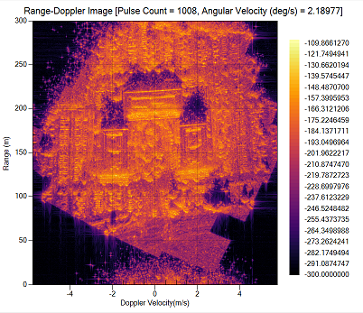
Radar image plot of RadarAnalysis1 at Time=50 epsec
Creating a movie of the scene
You can create a movie of the plots from all the steps between 30 epoch seconds to 70 epoch seconds in your results.
- Right-click the plot and select Export Movie. Its dialog box will appear.
- Change the Frame Rate to 2 fps so that the movie doesn't run too quickly.
- Make sure that the Open in associated viewer check box is selected. This will tell the RF Channel Modeler plugin that you want to open a video viewing app to see the movie immediately after you save it.
- Click .
- Give your movie a name and click .
- Watch your movie.
Viewing in the 3D Graphics window
You can see the radar image in the 3D Graphics window of the STK application.
- Minimize the RF Channel Modeler plugin UI. You should see the 3D Graphics window.
- Select Aircraft1 in the Object Browser.
- Right-click it and select Zoom To. You will see the helicopter up close.
- Zoom out some until you see the RadarAnalysis1 area.
- Locate the Animation toolbar. It has typical control buttons like Start, Pause, Step Forward/Back, etc.
- Click Start (
 ). You will see the Aircraft move along its flight path, with the radar transceiver tracking the Place object. At the 30-second mark, you will see the radar image appear in the analysis area. It will remain there until the 70-second mark.
Focusing on the radar image
If you want to focus on seeing the radar image change as the scenario unfolds, you can take some steps to clear up the 3D Graphics window and zoom in on the analysis area.
- In the Object Browser, clear the check box next to Sensor1. This will eliminate the cone going from Aircraft1 to the analysis area.
- Bring up the RF Channel Modeler UI again.
- In the Facet Tileset subtab of the Analysis tab, clear the Show Extent check box. This will make the yellow extents box disappear.
- Click at the bottom of the window to make these changes effective.
- Go to the Image Data Products subtab.
- Click in the lower-right corner. This will focus your view on the radar image as seen from the sensor for whatever instant in time you are at in the scenario.
- Minimize the RF Channel Modeler plugin UI.
- Set the animation toolbar time to start at 30 seconds. This is the start of your radar analysis.
- Reduce the speed of your animation by clicking the Decrease Time Step icon (
 ) twice to reduce the animation step size from 10 seconds to three seconds.
 - Click Start () and watch as the scenario steps through from 30 to 70 seconds.
You control the contrast and color scheme for this radar image using the Waterfall Properties button on Image Data Products tab of the RF Channel Modeler plugin UI, not from the Waterfall Properties options when right-clicking the plot in the Results tab.
Adding a scene contributor
Aircraft2 has a model with facets, so when you add it as a scene contributor, it will appear in the radar image just at the front edge of the courtyard. You will create a second analysis configuration to bring in this scene contributor without disturbing the original analysis configuration. Adding a scene contributors places a custom item in the analysis that can cause signal reflections, in addition to the reflections from existing objects and terrain in the facets tileset. The RF Channel Modeler plugin will check to assure that any scene contributor object you select has an associated model that provides suface facets, otherwise the analysis configuration will not be available to run.
Creating a second analysis configuration
You will create a second analysis configuration by copying the first. This second configuration will be the same as the first, with the difference being the addition of Aircraft2 as a scene contributor.
- Open the RF Channel Modeler plugin UI.
- Select RadarAnalysis1 at the top of the Analysis tab.
- Click the Duplicate Configuration icon (
 ).
). - Enter "RadarAnalysis2" as the Name in the Duplicate Configurations Analysis dialog box.
- Click to close the dialog box.
- Click at the bottom of the window to save these changes.
Adding the scene contributor
- Select RadarAnalysis2 at the top of the Analysis tab.
- Go to the Scene Contributor Objects subtab.
- Click the Add Scene Contributor icon () to open the Add Analysis Configuration Scene Contributors dialog box.
- Select Aircraft2 and click . Make sure that the Material for Aircraft2 is set to Metal.
- Click at the bottom of the window to save these changes.
- Click to compute the results with Aircraft2 now part of the scene.
Plotting the RadarAnalysis2 scene run results
Generate a plot of the data from running RadarAnalysis2.
- Select the Results tab at the top of the RF Channel Modeler UI. You should see the plot from RadarAnalysis1 left over from your previous activity.
- Select the Use analysis output folder as results folder check box, if not already selected, near the top of the Results tab. This tells the RF Channel Modeler to automatically point to the output folder specified in the Analysis tab.
- The Results Filter should default to the latest run. If not, make sure it is set for the RadarAnalysis2 run.
- Set the following under Plotting Parameters:
Extent parameter Value Transmit Antenna Index 0 Receive Antenna Index 0 Time Sample (EpSec) 50 - Click .
- You should see Aircraft2 appear at the front edge of the middle of the courtyard in your analysis scene.
Viewing just Aircraft2
You can remove the facet tileset of AGI Headquarters to show the radar image of just Aircraft2.
- Go to the Facet Tileset subtab of the Analysis tab.
- Select the AGI_Headquarters tileset.
- Click .
- Click at the bottom of the window to save these changes.
- Click .
- Go to the Results tab.
- Click . You should see just Aircraft2 and a very small dot at the center of the plot, which is Place1.
You can try out different plotting options with this view, including seeing the movie.
Saving your work
- Close the RF Channel Modeler plugin UI.
- Save () your work.
Summary
In this exercise, you learned how to use the STK application and the RF Channel Modeler plugin to do the following:
- Create an aircraft to fly by a scene, set a small object in the middle of the scene, and create a stationary aircraft on the ground, all in the STK application
- Place a Sensor object on the aircraft flying by the scene
- Use RF Channel Modeler to add transceivers to the Sensor object and apply specific antenna types, waveforms, and graphics properties to the transceivers
- Designate a radar transceiver for analysis configurations
- Include local structures, terrain, and scene contributors in the analysis
- Specify analysis extents
- Set radar product data parameters and generate radar plots to visualize your results data
- Make a movie of the resulting plot from each time step
On your own
In this lesson, you set up and ran two analysis configurations, with the only variation being a scene contributor. You could try placing the sensor (radar transceiver) on an object on the ground and imaging the aircraft flying by.
You can also explore using the STK Connect commanding capability to perform both the STK scenario setup and the RF Channel Modeler analysis configuring and execution. To do this, you should first complete the STK general tutorial on Connect commanding:
Level 1, Part 5: Introduction to Connect
This will help you on your way toward building the STK scenario. You can then set up and run RF Channel Modeler analysis configurations, perform the runs, and retrieve the results. Use the following Help pages to guide your building of the RF Channel Modeler plugin commanding:
RfChannelModeler - These are the basic commands for setting up and running analysis configurations.
RfChannelModeler_RM - Use these commands to retrieve information from the RF Channel Modeler plugin.
RfChannelModelerGraphics - Use this command to set values for graphics quantities such as antenna boundaries and analysis extents.
RfChannelModelerGraphics_RM - Use this command to retrieve values for graphics attributes.