STK Premium (Space) or STK Enterprise
You can obtain the necessary licenses for this tutorial by
The results of the tutorial may vary depending on the user settings and data enabled (online operations, terrain server, dynamic Earth data, etc.). It is acceptable to have different results.
Capabilities covered
This lesson covers the following capabilities of the Ansys Systems Tool Kit® (STK®) digital mission engineering software:
- STK Pro
- Space Environment and Effects Tool (SEET)
- Analysis Workbench
- Volumetric Analysis
Problem statement
Engineers and mission planners require a way to comprehensively model the space environment and the ambient near-Earth environment effects on space vehicles. They need to estimate the trapped energetic electrons and protons and how the thickness of a satellite's shielding affects radiation dosage for purposes of space system design and mission planning.
Solution
Use the STK software's Space Environment and Effects Tool (SEET) capability to determine the expected dosage rates and accumulated doses due to energetic electron and proton particle fluxes for a range of shielding thicknesses on a spacecraft. Configure scenario and spacecraft properties as needed to obtain low- and high-resolution dose depth and minimum / maximum flux comparisons. Use the Analysis Workbench and Volumetric Analysis capabilities to display Earth's radiation belts in 3D for visualization purposes.
What you will learn
Upon completion of this tutorial, you will be able to:
- Use Fast International Geomagnetic Reference Field coefficients for the geomagnetic field model
- Apply the local-time-dependent Olson-Pfitzer external field model
- Use multiple computational flux models for comparison
- Analyze radiation dose depth
- Analyze radiation flux
- Visualize Earth's radiation belts in 3D
Video guidance
Watch the following video. Then follow the steps below, which incorporate the systems and missions you work on (sample inputs provided).
Creating a new scenario
First, you must create a new scenario, and then build from there.
- Launch the STK application (
 ).
). - Click
 Create a Scenario in the Welcome to STK dialog box.
 - Enter the following in the STK: New Scenario Wizard:
- Click when you finish.
- Click Save (
 ) when the scenario loads. The STK application creates a folder with the same name as your scenario for you.
 - Verify the scenario name and location in the Save As dialog box.
- Click .
| Option | Value |
|---|---|
| Name | SEET_RadiationEnvironment |
| Location | Default |
| Start | Default |
| Stop | Default |
Save (![]() ) often during this scenario!
) often during this scenario!
Changing the scenario-level units of measure
- Right-click on SEET_RadiationEnvironment () in the Object Browser.
- Select Properties (
 ) in the shortcut menu.
 - Select the Basic - Units page.
- Select the Sort - Alphabetical option in the Dimension List panel.
- Scroll down and locate RadiationShieldThickness.
- Click the Mils (Mils) cell in the CurrentUnit column.
- Open (
 ) the drop-down list.
 - Select Millimeters (mm).
- Select the Enter key.
- Click to accept your selection and to close the Properties Browser.
Inserting a Satellite object
Use a Satellite object to model your spacecraft.
Inserting a new Satellite object using the Orbit Wizard
Use the Insert STK Objects tool to create a new Satellite object using the Orbit Wizard. The
- Bring the Insert STK Objects tool (
 ) to the front.
 - Select Satellite (
 ) in the Select An Object To Be Inserted list.
 - Select Orbit Wizard (
 ) in the Select A Method list.
 - Click .
Using the Orbit Designer
With the Orbit Designer option, you can create any orbit you wish. Use a nominal eccentric orbit that covers a large portion of the inner belt and a smaller portion of the outer belt, which will exercise the Radiation Environment models in the desired manner.
- Open the Type drop-down list in the Orbit Wizard.
- Select Orbit Designer.
- Enter Test_Sat in the Satellite Name field.
- Set the following in the Orbital Elements panel:
- Click to accept your changes, to propagate the satellite, and to close the Orbit Wizard.
| Parameter | Value |
|---|---|
| Semimajor Axis | 15000 km |
| Eccentricity | 0.4 |
| Inclination | 30 deg |
| Argument of Perigee | 50 deg |
| RAAN | 90 deg |
| True Anomaly | 0 deg |
Utilizing the SEET capability
The
Opening the satellite's SEET Environment properties
Configure the satellite's SEET environment on its
- Open Test_Sat's () Properties ().
- Select the Basic - SEET Environment page.
Setting the geomagnetic main field model
SEET uses a highly customizable set of conditions to compute the local magnetic field at the current location. The
- Open the Main Field drop-down list in the Magnetic Field Model panel.
- Select Fast IGRF.
For your analysis, you'll use the Fast IGRF option. The IGRF main field calculations are based on the full harmonic expansion IGRF coefficients. Fast IGRF is a specially tuned version of IGRF model that returns a field strength estimate accurate to within 1% of the full-IGRF option, but it is significantly faster.
Setting the external magnetic field model
Select the optional Olson-Pfitzer external field model for SEET. This model is based on Olson and Pfitzer's 1977 quantitative model of the magnetospheric field and associated procedures for accurately cataloging charged-particle data out to and beyond geosynchronous orbit. It only depends on the local time of one's position of interest within the field (that is, the position relative to the direction of the Sun).
- Open the External Field drop-down list.
- Select Olson-Pfitzer.
- Click to accept your selections and to keep the Properties Browser open.
Selecting the SEET radiation environment computational mode
The
Configure the SEET Radiation Environment for a long-time baseline dose depth analysis, after which you will generate the corresponding report. Since these generally take very long to compute, use the data-based models.
- Select the Basic - SEET Radiation page.
- Ensure the Computational Model is set to Radiation Only.
- Ensure the Dose Channel is set to Total.
- High LET: 1 - 10 MeV (particle energy) dosage, primarily from protons
- Low LET: 0.05 - 1 MeV, primarily from electrons, bremsstrahlung (electromagnetic radiation produced by the deceleration of a charged particle when deflected by another charged particle), with some high energy protons
- Total: uses both High LET and Low LET
- Enter 60 sec in the Dose Report Step field.
- Clear the Set magnetic field epoch to Mode's reference epoch check box.
- Click to accept your changes and to keep the Properties Browser open.
APEXRAD, CRRESRAD or Radiation-only (APEXRAD except where out of range of that model, in which case CRRESRAD is used) are fast, data-based models, but ones which have a limited range of shielding depths. They should be used for computationally fast, high-resolution dose-rate computations over long orbits. However, for access to the full range of SHIELDOSE-2 options (selectable depths, different detector types, species-resolved doses, greater spatial range of validity), either the CRRES or NASA models must be selected.
Dose Channel specifies which dose-rate data set to use. Linear energy transfer (LET) is the energy lost by an ion and deposited into the target material per unit distance along the ion’s path. This option only affects CRRESRAD and APEXRAD models.
This value specifies the default time step used by data providers reporting radiation-dose output.
In the Radiation Only, CRRESRAD and APEXRAD Computational Modes, only the prescribed sets of shielding thickness may be used.
Creating a SEET Radiation Dose Depth report
The
Duplicating the installed report style
You will duplicate the preinstalled SEET Radiation Dose Depth report and customize it from there.
- Right-click on Test_Sat () in the Object Browser.
- Select Report & Graph Manager... (
 ) in the shortcut menu.
 - Select the SEET Radiation Dose Depth (
 ) report in the Installed Styles (
 ) folder in the Styles panel of the Report & Graph Manager.
 - Click Duplicate style (
 ) in the Styles panel toolbar.
Changing the Shielding thickness report units and options
You want your report units to match the scenario units you set earlier. Both data providers use scientific notation by default, but you can make the report easier to read by setting the values to floating-point notation.
- Select the Content page.
- Select Shielding thickness in the Report Contents list.
- Click .
- Clear Use Defaults in the Units: Section 1, Line 1, Shielding thickness dialog box.
- Select Millimeters (mm) in the New Unit Value list.
- Click to accept your selection and to close the Units: Section 1, Line 1, Shielding thickness dialog box.
- Click .
- Open the Notation drop-down list in the Options: Section 1, Line 1, Shielding thickness dialog box.
- Select Floating Point.
- Click to accept your selection and to close the Options: Section 1, Line 1, Shielding thickness dialog box.
Changing the SEET Radiation Dose Depth - Combined dose report options
You also need to update the units for the Combined Dose to Floating Point.
- Select SEET Radiation Dose Depth - Combined Dose in the Report Contents list.
- Click .
- Open the Notation drop-down list in the Options: Section 1, Line 1, SEET Radiation Dose Depth - Combined dose dialog box.
- Select Floating Point.
- Click to accept your selection and to close the Options: Section 1, Line 1, SEET Radiation Dose Depth - Combined dose dialog box.
- Click to accept your selections and to close the Properties Browser.
Renaming the custom report
Although it's not required, it's a good idea to rename custom reports duplicated for an installed style.
- Right-click on the SEET Radiation Dose Depth (
 ) report in the My Styles () folder in the Styles panel.
 - Select Rename in the shortcut menu.
- Rename the SEET Radiation Dose Depth () report Custom SEET Radiation Dose Depth.
Generating the custom report
With your report configured, create and review the report.
- Select the Custom SEET Radiation Dose Depth () report.
- Click .
- Examine the data in the report.
- Close the report when finished.
- Leave the Report & Graph Manager open.
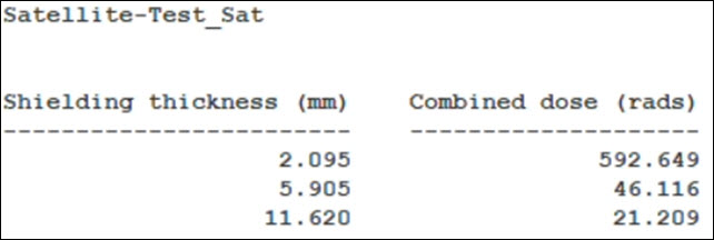
Custom SEET radiation dose depth report
The values will change depending on the date of your analysis
Using the CRRES flux model for high-resolution dose depth analysis
Configure the SEEET Radiation Environment for a high-resolution (i.e. many depths) dose depth analysis using the CRRES flux model. CRRES flux models are based on the CRRESELE and CRRESPRO models and are supported at discrete electron and proton energies based on data collected by the Combined Release and Radiation Effects Satellite's (CRRES) High Energy Electron Fluxmeter (HEEF) instrument (for omni-directional electron flux) and its PROTEL proton telescope (for omni-directional proton flux). Dose computations are performed by using the CRRES model results as input to SHIELDOSE-2.
Selecting the CRRES computational mode
Set the Computational Mode to use the CRRES flux model.
- Bring the Test_Sat's () Properties () to the front.
- Select the Basic - SEET Radiation page.
- Open the Computational Mode drop-down list in the Model panel.
- Select CRRES.
Selecting the detector geometry
Select the geometry of a material specimen under Aluminum shielding to be used for the dose computations. The default detector type is Silicon.
- Open the Detector Geometry drop-down list.
- Select Spherical.
A spherical detector is embedded at the center of a solid sphere of Aluminum and irradiated from all directions.
Setting the shielding thickness
You can specify up to 70 different Aluminum shielding thicknesses as needed. This option is effective when operating with the CRRES and NASA computational modes for arbitrary proton and electron incident spectra and used for dose computations from the SHIELDOSE-2 radiation-transport model.
- Click in the Shielding Thickness panel.
- Click .
- Enter 1 mm in the Value cell.
- Select the Enter key.
- Enter the following additional values:
- 2 mm
- 3 mm
- 4 mm
- 6 mm
- 8 mm
- 10 mm
- 15 mm
- Click to accept your selections and to keep the Properties Browser open.
Creating a custom SEET Radiation Dosage report
Using the same SEET Radiation Dose Depth data provider, you can build a custom radiation dosage report at the shielding thicknesses you specified.
Creating a new report style
Rather than duplicating an existing report, you'll create a new style from scratch.
- Return to the Report & Graph Manager.
- Select the My Styles () folder in the Styles panel.
- Click Create new report style (
 ) in the Styles panel toolbar.
 - Enter Custom SEET Radiation Dosage as the report name.
- Select the Enter key.
Selecting data providers and elements
- Select the Content page.
- Expand (
 ) the SEET Radiation Dose Depth () data provider.
 - Insert (
 ) the following data provider elements (
 ) into the Report Contents list:
 - Shielding Thickness: The shielding thickness at which the dose was computed.
- Electron Dose: The accumulated radiation dose due to electrons for the shielding thickness indicated, at the given time. Valid when using NASA or CRRES models.
- Electron Bremsstrahlung Dose: The accumulated radiation dose due to bremsstrahlung electrons, at the given time. Valid when using NASA or CRRES models.
- Proton Dose: The accumulated radiation dose due to protons for the shielding thickness indicated, at the given time. Valid when using NASA or CRRES models.
- Combined Dose: The accumulated total radiation dose from all constituents, at the given time.
Changing the Shielding thickness report units and options
You want to match your shielding thickness report units to match the scenario units you set earlier and its notation to be floating point.
- Select Shielding thickness in the Report Contents list.
- Click .
- Clear Use Defaults in the Units: Section 1, Line 1, Shielding thickness dialog box.
- Select Millimeters (mm) in the New Unit Value list.
- Click to accept your selection and to close the Units: Section 1, Line 1, Shielding thickness dialog box.
- Click .
- Open the Notation drop-down list in the Options: Section 1, Line 1, Shielding thickness dialog box.
- Select Floating Point.
- Click to accept your selection and to close the Options: Section 1, Line 1, Shielding thickness dialog box.
Changing the SEET Radiation Dose Depth - Electron dose report options
You can make the report easier to read by setting the dose values to floating-point notation.
- Select SEET Radiation Dose Depth-Electron dose in the Report Contents list.
- Click .
- Open the Notation drop-down list in the Options: Section 1, Line 1, SEET Radiation Dose Depth-Electron dose dialog box.
- Select Floating Point.
- Click to accept your selection and to close the Options: Section 1, Line 1, SEET Radiation Dose Depth-Electron dose dialog box.
Changing the SEET Radiation Dose Depth - Electron - Bremsstrahlung dose report options
Repeat the steps for the bremsstrahlung dose data.
- Select SEET Radiation Dose Depth-Electron-Bremsstrahlung dose in the Report Contents list.
- Click .
- Open the Notation drop-down list in the Options: Section 1, Line 1, SEET Radiation Dose Depth-Electron-Bremsstrahlung dose dialog box.
- Select Floating Point.
- Click to accept your selection and to close the Options: Section 1, Line 1, SEET Radiation Dose Depth-Electron-Bremsstrahlung dose dialog box.
Changing the SEET Radiation Dose Depth - Proton dose report options
Now, update the Proton dose Notation to floating point.
- Select SEET Radiation Dose Depth-Proton dose in the Report Contents list.
- Click .
- Open the Notation drop-down list in the Options: Section 1, Line 1, SEET Radiation Dose Depth-Proton dose dialog box.
- Select Floating Point.
- Click to accept your selection and to close the Options: Section 1, Line 1, SEET Radiation Dose Depth-Proton dose dialog box.
Changing the SEET Radiation Dose Depth - Combined dose report options
You want all of your dose depth data to be displayed in floating-point notation.
- Select SEET Radiation Dose Depth-Combined dose in the Report Contents list.
- Click .
- Open the Notation drop-down list in the Options: Section 1, Line 1, SEET Radiation Dose Depth-Combined dose dialog box.
- Select Floating Point.
- Click to accept your selection and to close the Options: Section 1, Line 1, SEET Radiation Dose Depth-Proton dose dialog box.
- Click to accept your selections and to close the Properties Browser.
Generating the custom report
With your report configured, create and review the report.
- Select the Custom SEET Radiation Dosage () report.
- Click .
- Examine the data in the report.
- Close the report when finished.
- Leave the Report & Graph Manager open.
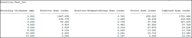
SEET Radiation dosage report
The values will change depending on the date of your analysis
Generating a Radiation Electron Flux graph
The SEET Radiation Flux data provider computes the radiation at each electron and proton energy level. The energy levels are determined by the computational mode; there are data items for electrons and protons at each of their respective energy levels, and the data are valid when using NASA or CRRES models. View these data as a graph.
- Bring the Report & Graph Manager to the front.
- Select the SEET Radiation Electron Flux (
 ) graph in the Installed Styles () list.
 - Click .
- Close the graph when finished.
- Leave the Report & Graph Manager open.
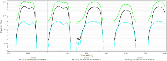
SEET Radiation electron flux graph (CRRES)
Using the NASA flux model
The NASA flux models cover a broad spatial and energy range but have been superseded by IRENE as the new industry standard. The CRRES models are based on a limited and specialized data set in the 1990s.
When using the NASA computational mode, flux models are based on NASA AE-8 radiation belt maps for electron flux for energies between 0.04 and 7.0 MeV, and NASA AP-8 radiation belt maps for proton flux for energies between 0.1 and 400 MeV. The calculations are performed by using the NASA model results as input to SHIELDOSE-2.
Selecting the NASA computational mode
Set the Computational Mode to use the NASA flux model.
- Bring Test_Sat's () Properties () to the front.
- Select the Basic - SEET Radiation page.
- Open the Computational Mode drop-down list in the Model panel.
- Select NASA.
- Click to accept your change and to close the Properties Browser.
Generating a new Radiation Electron Flux graph
Now that you've set the set the computational mode to NASA, generate a new SEET Radiation Electron Flux graph and view the changes.
- Bring the Report & Graph Manager to the front.
- Select the SEET Radiation Electron Flux () graph in the Installed Styles () list.
- Click .
- Close the graph when finished.
- Close the Report & Graph Manager.
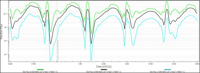
SEET Radiation electron flux graph (NASA)
Displaying Earth's radiation belts as a Volumetric object
Using the Analysis Workbench capability's Spatial Analysis tool and the Volumetric Analysis capability, you can view Earth's radiation belts in the 3D Graphics window. Volumetric Analysis involves evaluation of spatial conditions and calculations across a number of grid points. This analysis is configured in a Volumetric object, which also includes various 3D Graphics options such as display of grid points, and color and translucency of volumetric data.
Opening the Spatial Analysis tool
The
- Right-click on Test_Sat (
 ) in the Object Browser.
 - Select Analysis Workbench... (
 ) in the shortcut menu.
 - Select the Spatial Analysis tab in the Analysis Workbench.
Creating a new spatial calculation
Create a new spatial calculation. A Spatial Calculation is a calculation that depends on both time and location.
- Select Test_Sat () in the object tree.
- Click Create new Spatial Calculation (
 ) in the Spatial Analysis toolbar.
Defining a SEET Electron/Proton Radiation at Location spatial calculation component
Define your new
- Click Type - in the Add Spatial Analysis Component dialog box.
- Select SEET Electron/Proton Radiation At Location (
 ) in the Select Component Type list in the Select Component Type dialog box.
 - Click to accept your selection and to close the Select Component Type dialog box.
- Enter Electron 0.65 in the Name field.
- Keep the rest of the default settings.
- Click to accept your changes and to close the Add Spatial Analysis Component dialog box.
Creating a new volume grid
Create a new volume grid. A Volumetric grid is a collection of enumerated points placed in 3D space using steps taken in each coordinate using various coordinate types.
- Open the Filter by drop-down list.
- Select All Objects.
- Select Earth (
 ) in the object tree.
 - Click Create new Volume Grid (
 ) in the Spatial Analysis toolbar.
Creating a Cartographic grid
Select the Cartographic grid type. A Cartographic grid uses latitude, longitude and altitude based on the central body reference ellipsoid.
- Click Type - in the Add Spatial Analysis Component dialog box.
- Select Cartographic () in the Select Component Type list in the Select Component Type dialog box.
- Click to accept your selection and to close the Select Component Type dialog box.
- Enter Grid 1000 to 50000 km in the Name field.
- Note the default Central Body selection is Earth.
- Note the default Point Altitude selection of Altitude above Ellipsoid.
Earth is the central body for use as a reference for defining altitude.
The default ellipsoid is the WGS84 that is an Earth model with primary parameters defining the shape of an Earth ellipsoid.
Setting the volume grid values
Select and define the coordinate steps of the volume grid using a fixed number of steps. You'll specify the number of steps and set the minimum and maximum coordinate bounds.
- Click .
- Set the following in the Latitude panel of the Grid Values dialog box:
- Set the following in the Longitude panel:
- Set the following Altitude panel:
- Click to accept your changes and to close the Grid Values dialog box.
- Click to accept your changes and to close the Add Spatial Analysis Component dialog box.
- Click to close the Analysis Workbench.
| Option | Value |
|---|---|
| Latitude | Fixed Number of Steps |
| Minimum | -60 deg |
| Maximum | 60 deg |
| Number of Steps | 60 |
| Option | Value |
|---|---|
| Longitude | Fixed Number of Steps |
| Minimum | 0 deg |
| Maximum | 180 deg |
| Number of Steps | 18 |
| Option | Value |
|---|---|
| Altitude | Fixed Number of Steps |
| Minimum | 1000 km |
| Maximum | 50000 km |
| Number of Steps | 50 |
The number of steps determines how many points there are in the grid. The higher the number, the longer the calculation takes. Setting the longitude of 0 to 180 degrees will allow you to view a cross section of the grid.
Creating a new Volumetric object
A
- Insert a Volumetric (
 ) object using the Insert Default (
 ) method.
 - Open Volumetric1's () Properties ().
- Select the Basic - Definition page.
Selecting the volume grid
You will use the grid that you created using the Spatial Analysis tool.
- Click the Volume Grid ellipsis (
 ).
). - Select Earth (
 ) in the object tree in the Select Volume Grid for Volumetric1 dialog box.
 - Select Grid_1000_to_50000_km () in the Volume Grids for: Earth list.
- Click to accept your selection and to close the Select Volume Grid for Volumetric1 dialog box.
- Click to accept your changes and to keep the Properties Browser open.
Selecting the spatial calculation
You will use the spatial calculation that you created using the Spatial Analysis tool.
- Select the Spatial Calculation check box.
- Click the Spatial Calculation ellipsis ().
- Select Test_Sat () in the object tree in the Select Spatial Calculation for Volumetric1 dialog box.
- Select Electron_0.65() in the Spatial Calculations for: Test_Sat list.
- Click to accept your selection and to close the Select Spatial Calculation for Volumetric1 dialog box.
- Click to accept your changes and to keep the Properties Browser open.
- Save () your scenario.
Computing volumetric analysis
- Select Volumetric1 () in the Object Browser.
- Select Volumetric in the shortcut menu.
- Select Compute in the Volumetric submenu.
Changing Volumetric 3D Graphics attributes
The
- Return to Volumetric1's () Properties ().
- Select the 3D Graphics - Attributes page.
- Select the Smoothing check box.
- Click to accept your selection and to keep the Properties Browser open.
Changing the Volumetric 3D Graphics grid
The
- Select the 3D Graphics - Grid page.
- Clear the Show Grid check box.
- Click to accept your selection and to keep the Properties Browser open.
Changing the Volumetric 3D Graphics volume
The
- Select the 3D Graphics - Volume page.
- Select the Spatial Calculation Levels option.
- Click .
- Set the following in the Insert Evenly Spaced Values dialog box:
- Click .
- Click to accept your selection and to keep the Properties Browser open.
| Option | Value |
|---|---|
| Start | 1.25e10 |
| Stop | 2.25e11 |
| Step Size | 1.25e10 |
| Start Color | Red |
| Stop Color | Blue |
Creating a Volumetric 3D Graphics Legend
The
- Select the 3D Graphics - Legends page.
- Select the Fill Legend tab.
- Select the Show Legend check box.
- Enter Electron 0.65 MeV in the title filed in the Text Options panel.
- Enter 0 in the Number Of Decimal Digits field.
- Open the Notation drop-down list.
- Select Scientific (e).
- Enter 20 in the Max Color Squares per Row field in the Range Color Options panel.
- Enter 60 in the Color Square Width (pixels) field.
- Click to accept your changes and to close the Properties Browser.
While your reports and graphs were in floating-point notation, use scientific notation in your legend for legibility.
Viewing the volume in the 3D Graphics window
You can view the particle energy in the 3D Graphics window. You would have to create different spatial analysis components for different energy levels depending on which levels are the most important to you
- Bring the 3D Graphics window to the front.
- View the results.
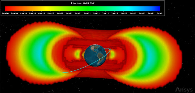
volumetric volume for 0.65 MeV
The low and high settings can be adjusted. Areas inside the volume lacking color are either below or above the original settings you used to create the volume colors.
Saving your work
Clean up your workspace and close out your scenario.
- Close any open reports and the Report & Graph Manager.
- Save () your work.
- Close the scenario when finished.
Summary
You created a scenario setting a satellite's SEET main field model to Fast IGRF, the external field model to Olson-Pfitzer and the computational mode to Radiation Only. Your first analysis was to use the default range of shielding thickness and running a report that analyzed the absorbed radiation dose. You changed the computational mode to CRRES and added multiple shielding thicknesses. You analyzed this using all the SEET Radiation Does Depth data provider elements. Next, you analyzed electron flux. Changing the computational mode to NASA you reanalyzed and viewed the differences in electron flux between CRRES and NASA. Finally, you used the Analysis Workbench to create a custom grid showing electron flux and applied the grid to the Volumetrics object that allowed you to visually see electron particle energy from 1,000 to 50,000 kilometers in the 3D Graphics window.