Numerical Integration |
Evaluating a definite integral, or more generally, evaluating the solution to an initial value problem (IVP), is often impossible or otherwise impractical analytically. Using numerical integration, we can approximate such a solution: that is, given an initial condition, we can take steps from an initial condition toward a desired endpoint, guided by the solution function's derivatives, and approximate the solution's value at each step. DME Component Libraries facilitates numerical integration with the NumericalIntegrator types, which fall into three families:
Integrators that extend RungeKuttaFixedStepIntegrator use a fixed step size when integrating.
Integrators that extend AdaptiveNumericalIntegrator adapt their step size to keep error under a certain threshold.
Integrators that extend MultipleStepIntegrator save multiple steps of derivative data to compute subsequent values more accurately.
Here we list the available NumericalIntegrator types. Note that many of these types specify an "order," which, unrelated to the order of the differential equation in the IVP, is simply a measurement of accuracy. In general, an nth-order algorithm whose current step size is h ensures that the current step's truncation error is on the order of h^n, where truncation error is the difference between the approximation and the exact solution at the end of the step, assuming there was no difference at the beginning of the step. For example, a fourth-order algorithm has a local truncation error on the order of h^4, indicating that using a step size of 0.5*h rather than h will decrease the error from E to (0.5)^4 * E for this step. In general, higher-order methods require more computation (specifically, more evaluations of the derivative) than lower-order methods.
NumericalIntegrator | Description |
|---|---|
A fourth-order fixed step Runge-Kutta integrator. | |
A fourth-order adaptive step Runge-Kutta algorithm that estimates error by comparing fourth and fifth-order approximations. | |
A seventh-order adaptive step Runge-Kutta algorithm that estimates error by comparing seventh and eighth-order approximations. | |
An adaptive step numerical integrator that estimates error as a function of step size: often an efficient choice for smooth systems, as opposed to discontinuous systems and systems with large variation in the derivatives. | |
A multi-step integrator based on the Gauss-Jackson algorithm, designed to efficiently integrate second-order equations. |
In the code below, we use a RungeKutta4Integrator to evaluate the following integral:

Equivalently, we evaluate the solution to the following IVP at x = 4.7.

We begin by defining an OrdinaryDifferentialEquationFunction to represent the system.
// Define a function that returns the array of derivatives of vector y, given y and
// its dependent variable x. Since our system is one-dimensional, y has length 1, and
// so does our return value.

private double[] derivative(double x, double[] y) {
    return new double[] { Math.cos(x) };
}
We then instantiate the system and the integrator.
// Instantiate a system by using the derivative function and specifying the order of the dependent variable (y) in the differential equation.
OrdinaryDifferentialEquationFunction function = OrdinaryDifferentialEquationFunction.of(this::derivative);
DependentVariableDifferentialEquation systemOfEquations = new DependentVariableDifferentialEquation(new OrdinaryDifferentialEquationSystem(function, 1));

// Instantiate a numerical integrator.
RungeKutta4Integrator rk4Integrator = new RungeKutta4Integrator(systemOfEquations);
Now we must ask ourselves what step size to use. While reducing step size reduces the truncation error for each step, it also requires us to take more steps to reach our endpoint. Therefore, we should choose a step size that allows us to approximate our solution to a desired level of accuracy without performing an unnecessarily large number of computations. In practice, we often choose a step size arbitrarily, then compare results with a smaller choice, perhaps half the chosen step size. In the following plot, we show results for one step, five steps, and ten steps.
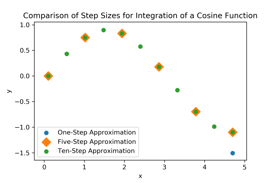
We immediately notice that one step is not accurate enough. When approximating at a point this far from the initial condition, it generally isn't.
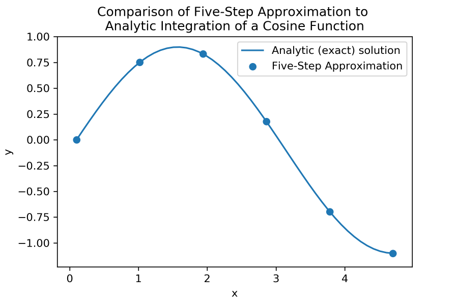
Meanwhile, there is no visual difference between the five and ten-step solutions, and we can verify numerically that the approximations at x = 4.7 differ by less than 0.001. This indicates that using more than five steps does not decrease our error by a significant amount. In the following plot, we see that five steps is a valid choice, accurately approximating the analytic solution.
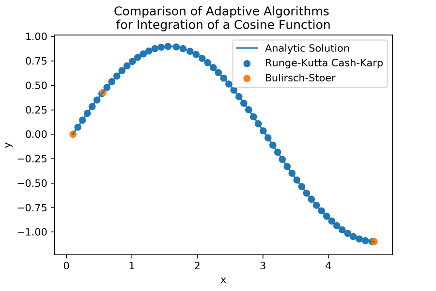
An alternative to manually determining step size is using an AdaptiveNumericalIntegrator, where we can specify the degree of accuracy we want to achieve and let the integrator determine the step size based on estimates of its own error at each step. In the following code, we use a RungeKuttaCashKarp45Integrator to solve the same IVP, specifying an accuracy of 1E-10.
RungeKuttaCashKarp45Integrator rkckIntegrator = new RungeKuttaCashKarp45Integrator(systemOfEquations, 0.1);

// Specify that we want to adapt step size to mitigate error.
rkckIntegrator.setStepSizeBehavior(KindOfStepSize.RELATIVE);

// Specify the tolerance we want to use.
rkckIntegrator.setAbsoluteTolerance(Constants.Epsilon10);

rkckIntegrator.initialize(0.1, new double[] { 0.0 });

while (rkckIntegrator.getFinalIndependentVariableValue() < 4.7) {
    rkckIntegrator.integrate();
}

// Since the while loop guarantees that we reached or overshot our desired endpoint (x = 4.7),
// we reintegrate with a specific step size to reach exactly 4.7. Since the step size
// here is guaranteed to be smaller than our last step (which overshot 4.7),
// our computed value is at least as accurate as the value computed for our last step.
rkckIntegrator.reintegrate(4.7 - rkckIntegrator.getInitialIndependentVariableValue());
y = rkckIntegrator.getFinalDependentVariableValues();
In this particular scenario, however, we know that our derivative function is relatively smooth on our interval of interest: that is, we aren't integrating a discontinuous function or a function with discontinuous derivatives. Therefore, we could opt to use a BulirschStoerIntegrator, as it is known to be a more efficient adaptive integrator for smooth functions. In the following plot, we see that if we repeat the above procedure for the same IVP with the same tolerance (1E-10) using a BulirschStoerIntegrator, we obtain a similar result to the RungeKuttaCashKarp45Integrator with far fewer steps.
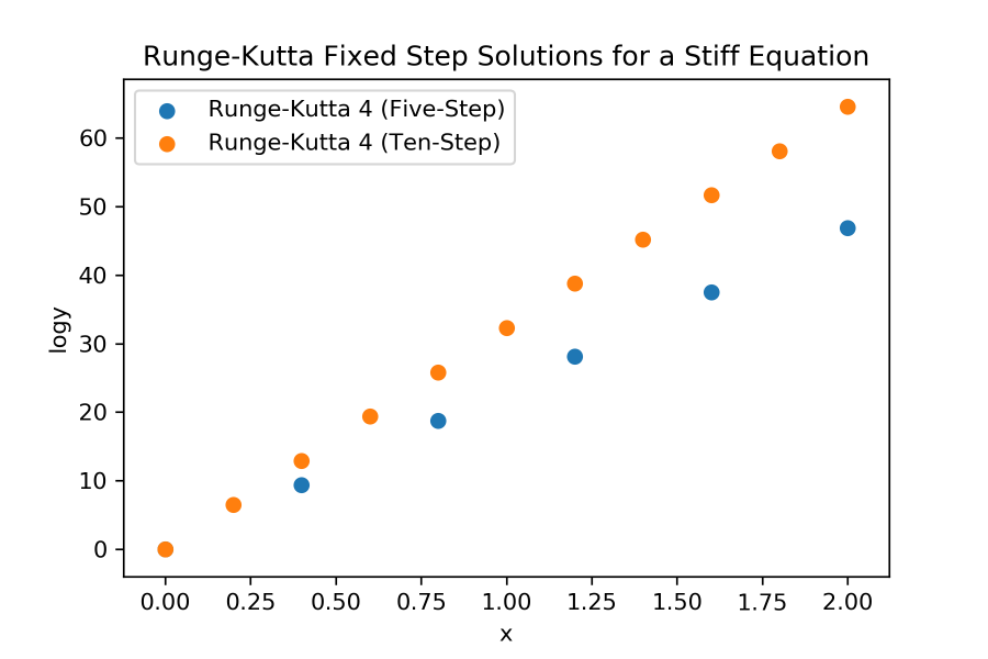
Just as in the case above, choice of method will often depend on the specific equation that we want to integrate, as well as the balance of efficiency and accuracy that we want to achieve. Making this choice can often be nontrivial. For example, consider the following IVP.

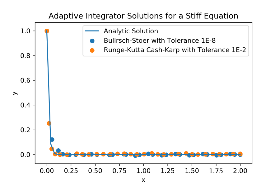
This equation belongs to a family of equations called "stiff" equations. While the literature on these equations is extensive, they can usually be recognized by extreme decay in their solutions, and they often cause Runge-Kutta methods to be unstable unless very small step sizes are used. In the following plot, where we attempt to solve at x = 2, we see that the RungeKutta4Integrator fails for multiple trial step sizes. The actual solution resides between 0 and 1 on the interval, while the approximations grow so large that we have to plot them on a logarithmic scale.
This is a case where determining step size by hand is impractical, and our best option is to choose between the available adaptive methods. As seen in the plot below, the Bulirsch-Stoer and Cash-Karp methods are both quite accurate, though again, the Bulirsch-Stoer algorithm uses fewer steps, even when set to a stricter tolerance. In practice, this can be controlled by modifying the MinimumStepSize (get / set) property, as adaptive integrators can often make their step sizes unnecessarily small.
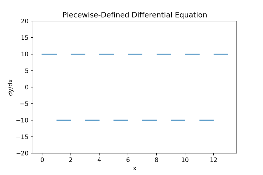
Bulirsch-Stoer is not always the best algorithm, of course. Consider an IVP defined piecewise as follows, along with the associated OrdinaryDifferentialEquationFunction. Here, 2Z refers to the set of even integers, and 2Z + 1 refers to the set of odd integers.

private double[] piecewiseDerivative(double x, double[] y) {
    if ((int) x % 2 == 0) {
        return new double[] { 10.0 };
    }
    return new double[] { -10.0 };
}
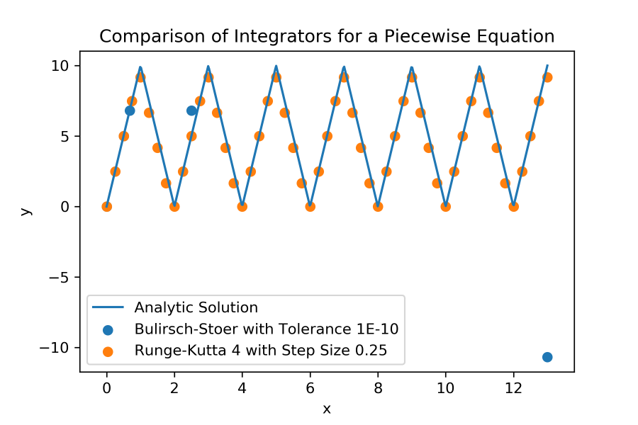
As mentioned before, Bulirsch-Stoer is quite efficient for smooth systems. In this case, however, our derivative is discontinuous, and when solving at x = 13, we see the algorithm perform quite poorly, while a RungeKutta4Integrator with step size 0.25 approximates quite well. In general, Bulirsch-Stoer is not suited for discontinuous and non-smooth systems.
The above paradigms can be extended, of course, to higher-dimensional systems. In the code below, we use a RungeKuttaFehlberg78Integrator to solve the following three-dimensional IVP at x = 61.1, where c = 1E-5:

// Define a function that returns the array of derivatives of vector y, given y and
// its dependent variable x.

private double[] derivatives(double x, double[] y) {
    return new double[] { y[0] * 1e-5 * x, y[1] * 1e-5 * x, y[2] * 1e-5 * x };
}
// Here we specify the order of each dependent variable (i.e. each component of y) in the differential equation.
function = OrdinaryDifferentialEquationFunction.of(this::derivatives);
systemOfEquations = new DependentVariableDifferentialEquation(new OrdinaryDifferentialEquationSystem(function, 1, 1, 1));

// Instantiate the integrator.
RungeKuttaFehlberg78Integrator rkfIntegrator = new RungeKuttaFehlberg78Integrator();
rkfIntegrator.setInitialStepSize(1);
rkfIntegrator.setStepSizeBehavior(KindOfStepSize.RELATIVE);
rkfIntegrator.setSystemOfEquations(systemOfEquations);

// Specify the initial conditions for the differential equation.
rkfIntegrator.initialize(0.1, new double[] { -1, 0.1, 3.124 });

while (rkfIntegrator.getFinalIndependentVariableValue() < 61.1) {
    rkfIntegrator.integrate();
}
rkfIntegrator.reintegrate(61.1 - rkfIntegrator.getInitialIndependentVariableValue());
y = rkfIntegrator.getFinalDependentVariableValues();
It is also possible to integrate higher-order systems, such as the following:

In the following code, we define the OrdinaryDifferentialEquationFunction by the second derivative of y's first component, and the first derivative of its second component. Here, g refers to the free-fall acceleration due to gravity near Earth's surface.
// Define a function that returns the first derivative of the first component of y and the
// second derivative of the second component of y, given y and its dependent variable x.
// Note the format of y: y1, y1', y2. In general, a dependent variable's derivatives' values
// immediately follow its own value.

private double[] secondOrderDerivatives(double x, double[] y) {
    return new double[] { -g, y[2] * 1e-5 * x };
}
After defining the derivative function, we integrate to x = 2 using a RungeKutta4Integrator.
// Here we specify that y's first component has order 2, and its second component has order 1.
function = OrdinaryDifferentialEquationFunction.of(this::secondOrderDerivatives);
systemOfEquations = new DependentVariableDifferentialEquation(new OrdinaryDifferentialEquationSystem(function, 2, 1));

// Instantiate the integrator.
rk4Integrator = new RungeKutta4Integrator(systemOfEquations);

// Specify initial conditions.
rk4Integrator.initialize(0.0, new double[] { 0.0, g, 0.1 });
rk4Integrator.integrate();
rk4Integrator.integrate();

y = rk4Integrator.getFinalDependentVariableValues();
In the above examples, we integrated explicit equations; in application, however, we might not have our system defined explicitly, but rather by data. In the next example, we solve the classic problem of finding the work done by a rocket that loses mass in the form of fuel as it ascends. First, we use numerical propagation to generate a point representing the rocket's motion on a 20 second interval, as well as evaluators for forces.
private static final JulianDate s_startDate = GregorianDate.parse("20000831T124242.00").toJulianDate();
private PointEvaluator m_pointEvaluator;
private ForceEvaluator m_gravityEvaluator;
private ForceEvaluator m_thrustEvaluator;
private ScalarEvaluator m_massEvaluator;
private static final double StepSize = 0.1;
private final void generateEvaluatorsFromPropagation() {
    CentralBody earth = CentralBodiesFacet.getFromContext().getEarth();

    // Create a newtonian point to store force models for the numerical propagator.
    PropagationNewtonianPoint newtonianPoint = new PropagationNewtonianPoint();
    newtonianPoint.setIdentification("myPoint");

    // Initialize the point approximately at the Earth's surface, at rest.
    newtonianPoint.setInitialPosition(new Cartesian(0.0, 0.0, 6.37e6));
    newtonianPoint.setInitialVelocity(new Cartesian(0.0, 0.0, 0.0));

    // Set the point's mass to a custom scalar that decreases with time, representing the rocket's fuel depletion.
    newtonianPoint.setMass(new MassScalar());

    ForceModel gravityModel = new TwoBodyGravity(newtonianPoint.getIntegrationPoint());
    ForceModel thrustModel = new ConstantForce(earth.getFixedFrame().getAxes(), new Cartesian(0.0, 0.0, 30e6));

    newtonianPoint.getAppliedForces().add(gravityModel);
    newtonianPoint.getAppliedForces().add(thrustModel);

    // Create a propagator and get a motion collection on a 20 second interval.
    NumericalPropagatorDefinition def = new NumericalPropagatorDefinition();
    final RungeKutta4Integrator rk4 = new RungeKutta4Integrator();
    rk4.setInitialStepSize(StepSize);
    def.setIntegrator(rk4);

    def.setEpoch(s_startDate);
    def.getIntegrationElements().add(newtonianPoint);

    NumericalPropagator propagator = def.createPropagator();
    NumericalPropagationStateHistory history = propagator.propagate(new Duration(0, 20.0), 1);
    DateMotionCollection1<Cartesian> motions = history.getDateMotionCollection("myPoint");

    // Get a point representing the propagation that we can use for later analysis.
    Point point = new PointInterpolator(earth.getFixedFrame(), InterpolationAlgorithmType.LINEAR, 1, motions);
    m_pointEvaluator = point.getEvaluator();

    // Get evaluators for later analysis.
    m_gravityEvaluator = new TwoBodyGravity(point).getForceEvaluator();
    m_thrustEvaluator = thrustModel.getForceEvaluator();
    m_massEvaluator = new MassScalar().getEvaluator();
}
Recall the following relationships between force, velocity, power, and work.


Using these relationships, we define our derivative function: that is, the power function.
// Recall that the derivative of work is power, i.e. force times velocity.
private double[] thrustPower(double t, double[] w) {
    JulianDate evalDate = s_startDate.add(new Duration(0, t));
    return new double[] { m_thrustEvaluator.evaluate(evalDate).dot(m_pointEvaluator.evaluate(evalDate, 1).getFirstDerivative()) };
}
Finally, we integrate to find the work done by the rocket at various times along a 10 second interval. We use a step size of 0.1 seconds, noting that when we use a step size of 0.05, the result at 10 seconds differs by about 12 joules. Therefore, we judge that the error is relatively small in comparison to the work values, which are on the order of billions.
generateEvaluatorsFromPropagation();

OrdinaryDifferentialEquationFunction function = OrdinaryDifferentialEquationFunction.of(this::thrustPower);
DependentVariableDifferentialEquation systemOfEquations = new DependentVariableDifferentialEquation(new OrdinaryDifferentialEquationSystem(function, 1));

RungeKutta4Integrator rk4Integrator = new RungeKutta4Integrator(systemOfEquations);
rk4Integrator.setInitialStepSize(StepSize);

// At t=0, the rocket hasn't done any work yet.
rk4Integrator.initialize(0.0, new double[] { 0.0 });

// Populate a list of work values along a 10 second interval.
ArrayList<Double> thrustWorks = new ArrayList<Double>();
for (int i = 0; i < 100; i++) {
    rk4Integrator.integrate();
    double[] w = rk4Integrator.getFinalDependentVariableValues();
    thrustWorks.add(w[0]);
}
We can find the work done by gravity in a similar manner.
private double[] gravityPower(double t, double[] w) {
    JulianDate evalDate = s_startDate.add(new Duration(0, t));
    // TwoBodyGravity is defined as a specific force, so we must multiply by mass to get the force in Newtons.
    return new double[] { m_massEvaluator.evaluate(evalDate) * m_gravityEvaluator.evaluate(evalDate).dot(m_pointEvaluator.evaluate(evalDate, 1).getFirstDerivative()) };
}
function = OrdinaryDifferentialEquationFunction.of(this::gravityPower);
systemOfEquations = new DependentVariableDifferentialEquation(new OrdinaryDifferentialEquationSystem(function, 1));
rk4Integrator = new RungeKutta4Integrator(systemOfEquations);
rk4Integrator.setInitialStepSize(StepSize);

rk4Integrator.initialize(0.0, new double[] { 0.0 });

ArrayList<Double> gravityWorks = new ArrayList<Double>();
for (int i = 0; i < 100; i++) {
    rk4Integrator.integrate();
    double[] w = rk4Integrator.getFinalDependentVariableValues();
    gravityWorks.add(w[0]);
}
While this example uses a constant thrust, the procedure is identical for a thrust that varies with time.
The choice of method and parameters for numerical integration is equation-specific, and it can often be a nontrivial choice, especially for stiff and non-smooth systems. The integrators provided should be sufficient for most problems, though obtaining accurate, efficient results can often be a trial-and-error process.