Modeling Propagation Loss in an Urban Environment
STK Professional, Communications, (Undefined variable: licenses.Coverage) and Urban Propagation Extension (UProp)
The results of the tutorial may vary depending on the user settings and data enabled (online operations, terrain server, dynamic Earth data, etc.). It is acceptable to have different results.
Watch the following video, then follow the steps below incorporating the systems and missions you work on (sample inputs provided).The main focus of this tutorial is how to make optimal use of the Urban Propagation Wireless InSite RT Model.
Install UProp
Urban Propagation Extension for STK Communications must be installed on your computer. In order to obtain an installation of UProp and a demo license, you will need to call 1.610.981.8875 or Email eval@agi.com.
Set the Scene
In the following tutorial, you will analyze communications between a command post and a patrol vehicle in a city environment. The analysis will include:
- A link budget between a transmitter at the command post and a receiver attached to the ground vehicle to assess the quality of the communications link while the ground vehicle travels through the urban environment.
- Computation of the signal strength throughout the operations area providing a quick overview of communication problem zones.
Urban Propagation Wireless InSite RT Model
The Urban Propagation Wireless InSite RT model offers a selection of a deterministic model and four empirical models for calculating path loss between two locations in an urban environment. The deterministic model, Triple Path Geodesic, is developed by Remcom, as a derivative of their Wireless InSite 3D propagation loss module, Wireless InSite Real Time.
Recommendations when using UProp:
| Option | Description |
|---|---|
| Frequency: | Frequency cannot go below 100 MHz. There is no upper limit restriction; however, above 7 GHz, predictions can become more sensitive to the finer resolution building details that may not be present in the shapefile or in the model's internal, simplified geometry. |
| Height Above Ground | Provided that both transmitter and receiver are above ground, there is no height restriction. However, prediction fidelity is reduced if both the transmitter and receiver are on or close to the ground (less than one meter) since ground conditions that are important to the analysis (e.g., ground cancellation) are not included. |
| Line of Sight and Az-El Mask constraints | It is recommended that you do not enable STK Line of Sight and Az-El Mask constraints. The Triple Path Geodesic model of the Urban Propagation Extension employs a higher-fidelity algorithm to simulate RF propagation in an urban environment than a simple line-of-sight prediction. In particular, the model has the capability to make signal attenuation predictions in situations where line-of-sight transmission is obscured, by considering three of the most significant paths of diffracted energy around buildings and over terrain. The use of Line of Sight and Az-El/terrain mask constraints is therefore not appropriate when using the Triple Path Geodesic model. |
A sample shapefile, Skopje.shp, used in this tutorial and is provided by East View Cartographic (EVC). For information on the recommended shapefile types, see Shapefile Requirements for the Urban Propagation Extension.
Create a Scenario
Start by creating a scenario.
- Launch STK (
 ).
). - From the Welcome to STK window, click Create a Scenario and enter the following:
- Click OK.
| Option | Value |
|---|---|
| Name | UProp_Tutorial |
| Analysis Period | Start time 1 Jul 2017 16:00:00.000 UTCG Stop + 5 min |
Save Often!
Use a Local Terrain File for Analysis
Add analytical terrain from a local file. Microsoft Bing Maps can be used for imagery. However, imagery is not required.
- Launch the Globe Manager (
 ) from the 3D Graphics window toolbar.
 - Use the Add Terrain/Imagery (
 ) option in the Globe Manager to load your terrain file (*.pdtt) both analytically and to the globe in the 3D Graphics window.
 - Browse to <Install Directory>Help\stktraining\samples and open SRTM_Skopje.pdtt.
- Click Yes when prompted to Use Terrain for Analysis.
Example install directory for STK 64 bit: C:\Program Files\AGI\STK 11\Help\stktraining\samples | Example install directory for STK 32 bit: C:\Program Files (x86)\AGI\STK 11\Help\stktraining\samples
Click here to learn how obtain urban terrain data.
Disable Terrain Server
You're using a local terrain file for analysis. Turn off Terrain Server.
- Open the UProp_Tutorial's (
 ) properties (
 ).
). - Browse to the Basic – Terrain page.
- Disable Use terrain server for analysis.
- Click Apply.
Set Urban Propagation Wireless InSite RT as the RF - Environment Loss Model
- Select the RF - Environment page.
- Click the Urban & Terrestrial tab.
- Enable Use.
- Select the Urban Propagation Wireless InSite RT as the Model Type.
- Ensure the TPDEODESIC is the Calculation Method. TPGEODESIC, which is the triple path compute option, produces higher fidelity results than the other options, which are empirical models.
- Select Enable Ground Reflection.
- Browse to the Urban building Geometry Data File (typically, <STK Install area>/Help/stktraining/samples).
- Select Skopje.shp.
- Select ZV2. The Building Height Data Attribute list contains all the columns in the data file. You will need to know which column contains the height attribute. In the Skopje.shp file, the ZV2 column contains the height attribute.
- Ensure Reference Method is set to HeightAboveTerrain.
- Enable Use Terrain Data.
- Click OK.
Declutter the 3D Graphics Window
Since you're using terrain in the 3D Graphics window, a common user preference is to use Label Declutter. It declutters labels away from the central body and towards the viewer, keeping the labels from being obscured by the terrain.
- Bring the 3D Graphics window to the front.
- Right-click on the 3D Graphics window and select Properties.
- On the Details page, find the Label Declutter field and check Enable.
- Click OK.
View the Skopje Shapefile
- Bring the 3D Graphics window to the front.
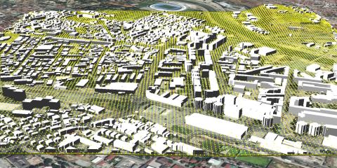
- In Globe Manager, right click on SRTM_Skopje.pdtt and select Zoom To. You can see the larger terrain file with the smaller Shapefile lying on top.
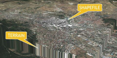
Terrain and Shapefile
Build the Command Post
Insert a Place object that will act as the command post.
- Using the Insert STK Objects Tool, insert a Place (
 ) object using the From City Database (
 ) method.
 - Enter Skopje in the Name: field and click Search.
- Select Skopje in the Results: field and click Insert.
- Close the Search Standard Object Data window.
- In the Object Browser, rename Skopje “Command_Post”.
- Open Command_Post's () Properties ().
- On the Basic - Position page, set Height Above Ground to one (1) m (one meter). This simulates a one-meter-tall antenna.
- Click OK.
Insert a Transmitter
Use a simple transmitter model.
- Insert a Transmitter object (
 ) using the Insert Default () method.
 - Attach the Transmitter () object to Command_Post ().
- Rename the Transmitter object "Cmnd_Xmtr."
- Open the Cmnd_Xmtr 's () properties ().
- On the Basic – Definition page, Model Specs tab, make the following changes:
- Select the Constraints - Basic page.
- Disable Line of Sight.
- Click OK.
| Option | Value |
|---|---|
| Frequency: | 5 GHz |
| EIRP: | 3 dBW |
Insert a Ground Vehicle
- Insert a Ground Vehicle object (
 ) using the Insert Default () method.
 - Rename the Ground Vehicle object "Test_Vehicle."
- Open the Test_Vehicle’s () properties ().
- In the Altitude Reference field, make the following changes:
- Click Insert Point and make the following changes:
- Click Insert Point four times make the following latitude/longitude changes in the following order starting with point two:
- Click OK.
| Option | Value |
|---|---|
| Reference: | Terrain |
| Terrain Granularity: | 1 m (meter) |
| Interp Method: | Terrain Height |
| Option | Value |
|---|---|
| Latitude | 42.00004 deg |
| Longitude | 21.41604 deg |
| Altitude | 1 m (meter) |
| Speed | 20 mi/hr |
| Latitude | Longitude |
|---|---|
| 41.99817 deg | 21.42527 deg |
| 42.00037 deg | 21.42708 deg |
| 41.99896 deg | 21.42978 deg |
| 41.99930 deg | 21.43370 deg |
Insert a Receiver
Use a simple receiver model.
- Insert a Receiver object (
 ) using the Insert Default () method.
 - Attach the Receiver object to Test_Vehicle ().
- Rename the Receiver object "Vehicle_Rcvr."
- Open the Vehicle_Rcvr 's () properties ().
- Select Constraints – Basic page.
- Disable Line of Sight.
- Click OK.
Insert an Area Target
Use an Area Target object to create a visual reference of the shapefile in the 2D and 3D Graphics windows.
- Insert an Area Target (
 ) object using the Area Target Wizard (
 ) method.
 - Change Name: to Test_Area.
- Click Insert point and make the following changes:
- Click Insert Point three times make the following latitude/longitude changes in order starting with point two:
- Click OK.
- Open Test_Area’s () properties ().
- Select the 3D Graphics – Attributes page.
- Enable Show Boundary Wall.
- Upper Edge: Height from Terrain / 10 ft (feet)
- Lower Edge: Height from Terrain / 0 km (kilometers)
- Click OK.
- Bring the 3D Graphics window to the front and zoom to Test_Area.
| Latitude | Longitude |
|---|---|
| 41.9904 deg | 21.4157 deg |
| Latitude | Longitude |
|---|---|
| 41.9904 deg | 21.4357 deg |
| 42.0044 deg | 21.4357 deg |
| 42.0044 deg | 21.4157 deg |
By setting the upper and lower edge of the boundary wall to Height from Terrain, it is easier to visualize the area target boundary on the map.
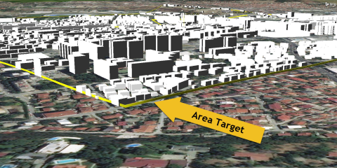
Area Target Boundary
Generate a Simple Link Budget
First, focus on the carrier to noise ratio (C/N) between the test vehicle and the command post. You can use a simple link budget to view the C/N.
- In the Object Browser, right-click on Vehicle_Rcvr () and select Access (
 ) to open the Access Tool.
 - In the Access Tool's Associated Objects List, expand (
 ) Command_Post.
 - Select Cmnd_Xmtr ().
- In the Reports field, click the Link Budget button.
- When the link budget report opens, go to Step: click Show Step Value and change Step: to 1 sec (second).
- Scroll to the right in the report and locate the C/N (dB) column.
- Scroll down the column. You can see the C/N fluctuate due to the effect of terrain (SRTM_Skopje.pdtt) and buildings (Skopje.shp) on the signal.
- When finished, close the report and the Access Tool.
A higher frequency will produce greater losses. If you test this and are taking the L3 Grand Master Certification, make sure you put the frequency back to 5 GHz.
Compute Object Coverage
- In the Object Browser, right-click Vehicle_Rcvr () and select Coverage.
- In the Assets window select Cmnd_Xmtr ().
- Click Assign.
- Click Compute.
- In the Figure of Merit field click Define.
- Make the following Definition changes:
- Click OK.
| Option | Value |
|---|---|
| Type: | Access Constraint |
| Constraints: | C/N |
| Across Assets: | Use Default |
| Compute: | Maximum |
Note the value in the Value: field. This is the maximum C/N dB value along the test vehicle's route.
Create a Graph
- In the Graphs field, click FOM Value.
- When the FOM Value graph opens, go to Step: click Show Step Value and change Step: to 1 sec (second).
- Close the graph.
The graph shows the C/N fluctuation as the test vehicle drives through the city. The approximate C/N values range from -10 (dB) to 92 (dB).
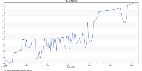
C/N dB Graph
Create Contours
You can apply color contours along the vehicle route which correspond to the C/N fluctuations.
- In the Figure of Merit field, click Contours.
- In the Level Adding field, make the following changes:
- Click Add.
- Enable Use Color Ramp.
- Change the Select ramp colors: to red and blue.
- Change Line Width: to the heaviest line width.
- Click Apply.
- Click the Legend… button.
- Click OK.
| Option | Value |
|---|---|
| Start: | -10 dB |
| Stop: | 90 dB |
| Step: | 10 dB |
View the Contours
- Bring the 3D Graphics window to the front.
- Resize the legend so that you can see all the numbers.
- Zoom in to the area target so that you can see the entire ground vehicles route.
- In the Animation Tool, decrease the time step to 0.10 sec (second).
- Click Start to view the ground vehicle as it travels through the city. Note the color changes based on C/N fluctuations.
- When finished, click the Reset (
 ) button.
 - Close the Legend.
- Return to the Coverage Tool and click Cancel.
- In the Object Browser, disable Test_Vehicle.
If the vehicle won't animate, close the legend. You can also see the results in the 2D Graphics window.
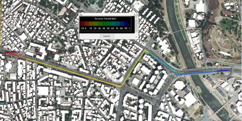
Vehicle Route
Compute Area Coverage
Use a Coverage Definition object to determine C/N in the operations area.
- Insert a Coverage Definition (
 ) object using the Insert Default () method.
 - Rename the Coverage Definition object “Area_Cov.”
- Open Area_Cov’s () properties ().
- On the Basic – Grid page, change Grid Area of Interest Type: to Custom Regions.
- Click the Select Regions button.
- Move Test_Area to the Selected Regions field.
- Click OK.
- Change Point Granularity, Lat/Lon to 0.0001 deg (degrees).
- Change Point Altitude to Altitude above Terrain and set the value to 1 m (meter).
- Click Apply.
View the Grid
- Bring the 3D Graphics window to the front to view the coverage grid.
Coverage Grid
Constrain the Grid
Use Vehicle_Rcvr to constrain the coverage grid.
- Return to Area_Cov's () properties ().
- Click the Grid Constraints Options button.
- Change Reference Constraint Class: to Receiver.
- Select Test_Vehicle/Vehicle_Rcvr in the Use Object Instance field.
- Click OK.
- Click Apply.
Select the Asset
- Select the Basic - Assets page.
- In the Assets field, select Cmnd_Xmtr.
- Click Assign.
- Click Apply.
One Second Computing
Since you're computing a static grid with no moving parts, you can decrease the time it takes to analyze the grid by decreasing the interval.
- Select the Basic - Interval page.
- Open the Interval pull down menu.
- Select Replace With Times.
- Change Stop: to "+ 1 sec" (second).
- Click Apply.
Automatically Recompute Accesses
If checked, STK automatically recomputes accesses every time an object on which the coverage definition depends (such as an asset) is updated. If you are making numerous property changes, you may want to turn this off.
- Select the Basic - Advanced page.
- Disable the Automatically Recompute Accesses option.
- Click Apply.
Disable the Visual Grid
Each grid point is shown in the 2D and 3D Graphics window as coverage computations are completed. If you are using color contours to visualize your coverage, you may want to remove the grid.
- Select the 2D Graphics - Attributes page.
- Disable the Show Points option.
- Click OK.
Insert a Coverage Figure of Merit
Insert a Coverage Figure of Merit object and configure it to analyze the C/N inside the test area.
- Insert a Figure Of Merit (
 ) object using the Insert Default () method.
 - When the Select Object window appears, select Area_Cov.
- Click OK.
- Rename the Figure Of Merit object "HowsMyCov."
- Open HowsMyCov's () properties ().
- On the Basic - Definition page, make the following changes:
- Click OK.
| Option | Value |
|---|---|
| Type: | Access Constraint |
| Constraints: | C/N |
| Across Assets: | Use Default |
| Compute: | Maximum |
Compute Coverage
- In the Object Browser, select Area_Cov ().
- Open the CoverageDefinition menu.
- Select Compute Accesses.
Grid Stats
The Grid Stats report summarizes the minimum, maximum and average static value for the Figure Of Merit over the entire grid.
- In the Object Browser, right click HowsMyCov () and select the Report & Graph Manager (
 ).
). - In the Styles list, generate a Grid Stats report.
- Note the Minimum (dB) and Maximum (dB) values at the bottom of the report.
- Close the report and the Report & Graph Manager.
Be patient. The grid contains a lot of points (~ 26244) and may take a few minutes to generate the report.
Create Contours
For your purposes, you are only interested in a C/N of -100 dB to the maximum dB value noted in the Grid Stats report.
- Open HowsMyCov's () properties ().
- Select the 2D Graphics - Static page.
- Change % Translucency to 20 (percent).
- Enable Show Contours.
- In the Level Adding field, make the following changes:
- Click Add Levels.
- Change the Color Ramp colors to:
- Enable Natural Neighbor Sampling.
- Click Apply.
- Click the Legend Button.
- When the legend opens, click the Layout button.
- Change Title: to C/N dB.
- Change Number Of Decimal Digits to 0 (zero).
- Click OK.
- Resize the legend so that you can see all the values.
- Bring the 3D Graphics window to the front.
- When finished, close the Legend and HowsMyCov's () properties ().
| Option | Value |
|---|---|
| Start: | -100 dB |
| Stop: | round down to the nearest integer (e.g. 115) |
| Step: | 20 dB |
| Option | Value |
|---|---|
| Start: | Red |
| Stop: | Blue |
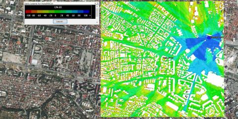
Static Coverage
Any areas in the map void of color have a C/N dB value less than -100 dB.
On Your Own
To change the coverage for either the test vehicle or the test area, you can raise the antenna height (Command_Post). You can try increasing or decreasing Cmnd_Xmtr's frequency and/or EIRP.
Save Your Scenario!
 Visit AGI.com