STK Premium (Air), or STK Enterprise
You can obtain the necessary licenses for this training by contacting AGI Support at support@agi.com or 1-800-924-7244.
Additional installation - STK's Electro-Optical Infrared Sensor Performance capability. You can obtain the necessary install by visiting http://support.agi.com/downloads or calling AGI support.
The results of the tutorial may vary depending on the user settings and data enabled (online operations, terrain server, dynamic Earth data, etc.). It is acceptable to have different results.
If you have not completed Parts 1 and 2 of the DME lessons, starter scenarios are provided. It requires STK 12 or newer to open. The DME lessons are in the Training - Level 3 - Focused tutorials section of the STK Help.
Capabilities Covered
This lesson covers the following STK Capabilities:
- STK Pro
- Communications
- Analysis Workbench
- Aviator
- Aviator Pro
- Electro-Optical Infrared Sensor Performance (EOIR)
Overview
Problem Statement
Across the industry, the digital engineering process is becoming more complex. Systems of systems are changing and updating in different stages of the mission lifecycle. In this series, we will address these challenges by creating a fully connected digital thread with a common mission environment at the core. We will design and test a new satellite constellation for persistent, stereo coverage of hypersonic vehicles across the world. We will discuss this topic in stages: satellite constellations, hypersonic flight, EOIR synthetic sensors, communications links, and triggering events and systems. Our vision is to integrate the mission environment and operational objectives into the digital thread early and throughout the entire product lifecycle. Through digital mission engineering, we are now capable of quickly evaluating the overall mission impact of the smallest change to any component. This session will look at event-based operations for mission or test and evaluation planning. We will be building on the previous scenarios to evaluate the series of events within a mission and how their dependencies on each other influence the overall mission effectiveness.
Solution
In this section of the Digital Mission Engineering (DME) series, we will focus on the test or mission planning phase of the lifecycle. Using the same models constructed through the design phase, we will evaluate relationships between assets like communications link availability and how that influences the overall mission timeline.
The communication system will be an important factor in the system response time of a detection and tracking system. Once we figure out how well our communication system works and which satellites are doing the communicating, we will discuss the system response time of the mission as a whole.
Upon completion of this tutorial, you will be able to:
- Build and analyze a communication link.
- Apply external antenna gain pattern files.
- Generate a Link Budget.
- Understand the series of events taking place.
- Link the relevant events together.
- Understand the system as a whole.
External Files
This lesson requires several external files:
- DME_Session3_Starter_Comms.vdf - This is the starter scenario for the STK Communications capability portion of this lesson
- DME_Session3_Starter_AWB.vdf - This is the starter scenario for the event and time components portion of the DME series
- stss.mdl - This is the custom satellite model
- SatCom_Omni_2p2G_Isolated.pattern - Simple antenna model to be loaded into the scenario
- SatCom_Omni_2p2G_Installed.pattern - Antenna model using ANSYS tools to account for absorption / reflection off the satellite body
The external files are available for download from the STK Data Federate, AGI - Document Library- STK 12 - Starter Tutorials - DME_Session3_Comms_and_Event_Analysis.
Video Guidance
Watch the following video. Then follow the steps below, which incorporate the systems and missions you work on (sample inputs provided).
Open a Starter Scenario
We built a starter scenario for you that contains the flight and the Pegasus hypersonic vehicle. You can open the scenario from the SDF or from a local copy, the downloaded scenario from the SDF or the completed scenario from DME: Hypersonics and EOIR (Part 2 of 3) Lesson.
Choose one of the three methods below to open a starter scenario.
Sign in to access the SDF
You can access your scenarios or objects from the STK Data Federate (SDF).
- Click (
 ) in the Welcome to STK dialog box.
 - Change the Location: to STK Data Federate at the bottom of the Open dialog window.
- Click Guest in the top right corner to sign into your account.
- Click when the SDF Server Login dialog box opens.
- Enter your Account name and Password on the Log In: AGI SEDS dialog box.
- Click .
Option 1: Open a Starter Scenario From the SDF - Use the Browse Method
If you want to open the starter scenario from the SDF, you can open it by browsing to the VDF file.
- Select the Browse tab.
- Navigate to Sites/AGI/documentLibrary/ STK 12/Starter Tutorials/DME_Session3_Comms_and_Event_Analysis
- Select DME_Session3_Starter_Comms.vdf.
- Click .
Option 2: Open a Starter Scenario From the SDF - Use the URL
If you want to open the starter scenario from the SDF, you can open it by copying and pasting the VDF's URL. The URL is https://sdf.agi.com/share/page/site/AGI/document-details?nodeRef=workspace://SpaceStore/f6d6ccf2-88e2-4ae0-b0ac-9b32ea1217ef
- Copy the following url: https://sdf.agi.com/share/page/site/AGI/document-details?nodeRef=workspace://SpaceStore/f6d6ccf2-88e2-4ae0-b0ac-9b32ea1217ef
- Right-click in the File name: field.
- Select Paste.
- Select DME_Session3_Starter_Comms.vdf.
- Click .
Option 3: Open a Starter Scenario Locally
If you want to open the starter scenario from a local file, follow the steps below.
- Click the Open a Scenario () button.
- Ensure STK User is selected on the left side of the Open window.
- Browse to the location of the saved starter scenario.
- Click .
Examine the scenario. Note that this mission is a continuation of what was built in DME: Hypersonics and EOIR. In the scenario, you should see the hypersonic test flight. Later in this mission, you can assess a system detecting and tracking the hypersonic aircraft.
Save Your Scenario
First you want to save your scenario. The way to save your scenario varies slightly depending if you opened the starter scenario from the SDF or from a local file.
Choose the appropriate save method below based on how you opened the starter scenario.
Option 1: Save Your Scenario After Opening It From the SDF
If you opened the starter scenario from the SDF, follow the steps below to save your scenario.
- Click File on the menu bar.
- Select Save As...
- Select STK User on the left side of the Save As window.
- Select DME_Session3_Starter_Comms folder.
- Click .
- Change Save as type: to Scenario Files (*.sc).
- Ensure the File name is X43_Mission_Comms.sc.
- Click .
- Click . to replace the existing file.
Option 2: Save Your Scenario After Opening It From a Local File
If you opened the starter scenario from a local file, follow the steps below to save your scenario.
- Click File on the menu bar.
- Select Save As...
- Select STK User on the left side of the Save As window.
- Click Create New Folder icon.
- Name it X43_Mission_Comms.
- Select the X43_Mission_Comms folder.
- Click .
- Ensure the Save as type: is Scenario Files (*.sc).
- Set the File name: to X43_Mission_Comms.sc.
- Click .
Create a Ground Station
The focus of this section is to create a communication system. You can begin creating the communication system by building a ground station. The ground station houses the receiver. The satellite communicates with the ground station receiver and you can use it to compare the coverage between the antenna models.
- Bring the Insert STK Objects tool (
 ) to the front.
 - Insert an Facility object (
 ) using the Define Properties (
 ) method.
 - Select the Basic - Position page.
- Set the following options:
- Click .
- Rename the ground site GroundTerminal.
- Save (
 ) the scenario.
| Option | Value |
|---|---|
| Latitude | 34.1084 deg |
| Longitude | -119.065 deg |
| Use terrain data | On |
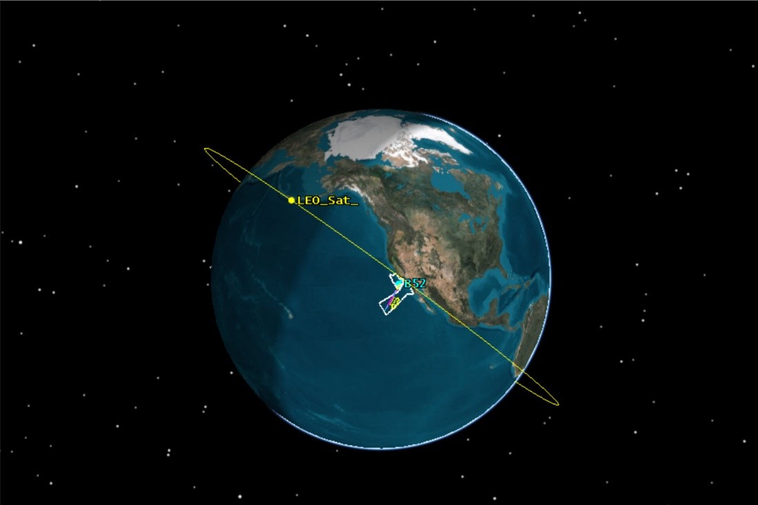
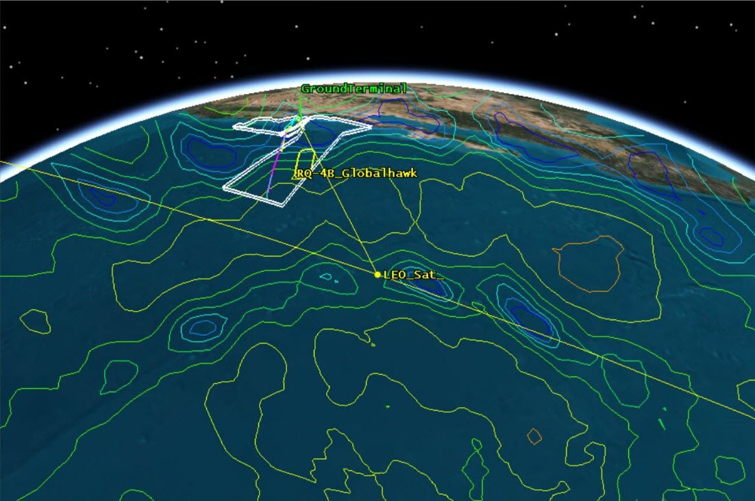
This location corresponds to Comms Terminals near Port Magu.
View in 3D
- Right-click on GroundTerminal () in the Object Browser.
- Select Zoom To.
- Mouse around the 3D Graphics window to understand the location of the ground terminal.
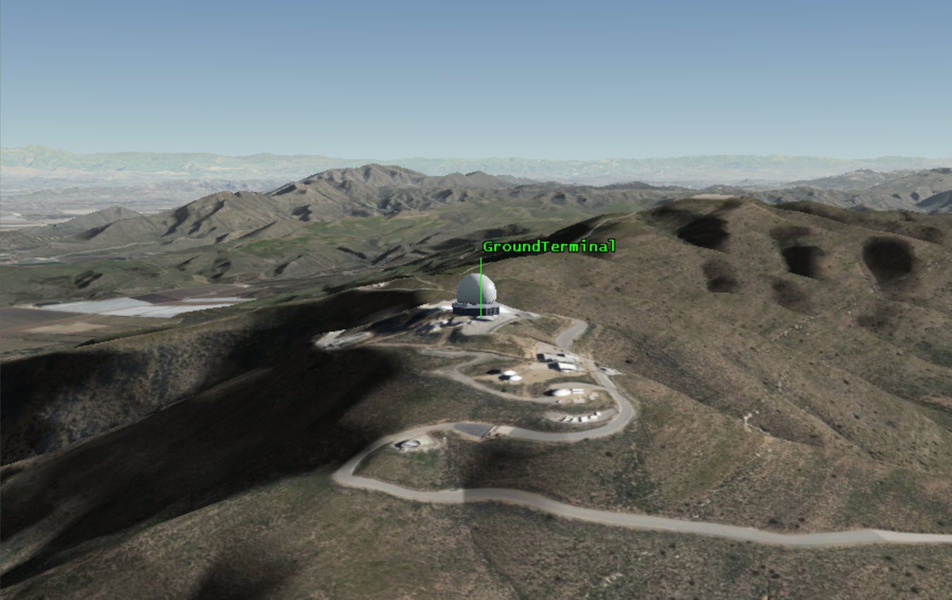
3D View: Ground Terminal
Create a Ground System Receiver
The ground system is receiving signals from all the satellites traveling overhead. Therefore, the receiver model is omnidirectional. This is modeled with a simple receiver that auto-tracks to all frequencies.
- Bring the Insert STK Objects tool () to the front.
- Insert an Receiver object (
 ) using the Insert Default () method.
 - Select GroundTerminal () in the Select Object window.
- Click .
- Rename the receiver Receiver.
- Save () the scenario.
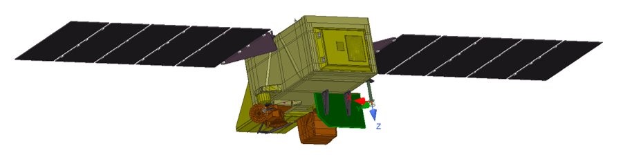
Create a Satellite to Mount the Transmitter
The satellite is the vehicle for the transmitter. It also functions as a seed satellite for a satellite constellation you set up later.
- Insert a Satellite (
 ) using the Orbit Wizard (
 ) method.
 - When the Orbit Wizard opens, set the following:
- Select the 3D Graphics - Model page.
- Click the ellipsis (
 ) beside the 3D Model field.
 - Browse to the location of the saved satellite model file.
- Select stss.mdl.
- Click .
- Save () the scenario.
| Option | Value |
|---|---|
| Type | Circular |
| Satellite Name | LEO_Sat |
| Inclination | 50 deg |
| Altitude | 1734 km |
The orbital values were found from another optimization of the satellite constellation. After the initial study in DME: Constellation Design, the parameters for the mission were updated and a new constellation for the system was designed. You can use this satellite to seed the constellation later in this lesson.
View in 3D
- Open the View From/To (
 ) drop-down.
 - Extend the Central Bodies menu.
- Select Earth.
- Animate (
 ) the scenario to view the satellite moving overhead.
Add a Transmitter to Model Accessibility
You can now begin by building the communication system. Initially, you want to model a simple omni-directional transmitter and analyze the communications link.
- Bring the Insert STK Objects tool () to the front.
- Insert an Transmitter object (
 ) using the Define Properties () method.
 - Select LEO_Sat () in the Select Object window.
- Set the Frequency to 2.2 GHz (This is a short range S-Band frequency).
- Click .
- Rename the transmitter Transmitter.
- Save () the scenario.
Compute the Link Budget to the Ground Terminal
First you can generate a link budget using the simple transmitter model and then update with a unique antenna pattern.
- Right-click on Transmitter () in the Object Browser.
- Select the Access... option.
- Expand GroundTerminal ().
- Select Receiver ().
- Click the Link Budget... button.
- Save the Link Budget as a quick report (
 ).
). - Save () the scenario.
This generates communication values between the two objects (GroundTerminal's Receiver and Satellite's Transmitter). You can see various values, like Carrier to Noise (C/N) Ratio. For this case, you are primarily going to look at the Bit Error Rate (BER) as the quality metric. This shows that for this case as long as line-of-sight is maintained, any sort of signal can be maintained. BER is effectively zero. This is primarily because you have a very simple transmitter.
Model the External Antenna
With an omni-directional, a simple transmitter, you can get an initial analysis of the satellite communications system. With DME in mind, you can modify your system and see how things change when you load an external antenna model in the scenario.
- Bring the Insert STK Objects tool () to the front.
- Insert an Antenna object (
 ) using the Define Properties () method.
 - Select LEO_Sat in the Select Object window.
- Click .
Define an External Antenna Pattern
- Select the Basic - Definition page.
- Set the Type to External Antenna Pattern.
- Set the Design Frequency 2.2 GHz.
- Click the ellipsis () button.
- Browse to the location of the pattern file.
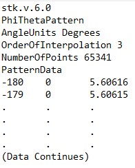
- Open the SatCom_Omni_2p2G_Isolation.pattern.
Pattern File
- Open the Pattern file in a text editor.
- Click Open.
- Click .
The pattern file is isolated from the body of the vehicle it is attached. This external antenna pattern could be provided by a third party, like a test lab. It could also be defined in another document, like a *.csv file. In order to turn this into an antenna gain pattern for STK, use Notepad and ensure the following header to the data.
			stk.v6.0
			PhiThetaPattern
			AngleUnits Degrees
			OrderOfInterpolation 3
			NumberOfPoints 65341 (note: this varies with your data set)
			PatternData
STK works well with the Phi-Theta sweep pattern of data. STK supports a wide variety of industry antenna gain formats. Contact support@agi.com if you have questions about other formats.
Orient the Antenna
By default, STK places the antenna in a fixed 90 deg elevation on the satellite. You can reorient it and change the position of the antenna. Realistically the antenna is not placed on the center of the model.
- Select the Basic - Orientation page.
- Set the following options:
- Set the following Position Offset values:
- Click .
| Option | Value |
|---|---|
| Azimuth | 270 deg |
| Elevation | 90 deg |
| Option | Value |
|---|---|
| X | -0.57 m |
| Y | 0.93 m |
| Z | 0.55 m |
Display the Contour Graphics
- Select the 2D Graphics - Contour page.
- Enable the Show Contour Graphics window.
- Locate the Level Adding field.
- Set the following options:
- Click the Add Level button.
- Disable the Relative to Maximum.
- Click .
| Option | Value |
|---|---|
| Start | -10 |
| End | 11 |
| Step | 3 |
Set the 3D Graphics Attributes
- Select the 3D Graphics - Attributes page.
- Enable the Show Lines option.
- Enable the Show Volume option.
- Set the following options:
- Click .
- Rename the antenna OmniIsolated.
- Save () the scenario.
| Option | Value |
|---|---|
| Gain Scale | 4 cm |
| Minimum displayed gain | -30 dB |
| Elevation Stop | 180 deg |
View in 3D
- Right-click on LEO_Sat () in the Object Browser.
- Select Zoom To.
- Mouse around the 3D Graphics window to understand the antenna pattern.
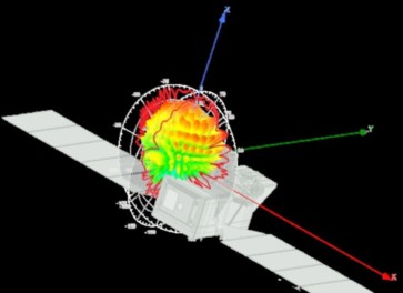
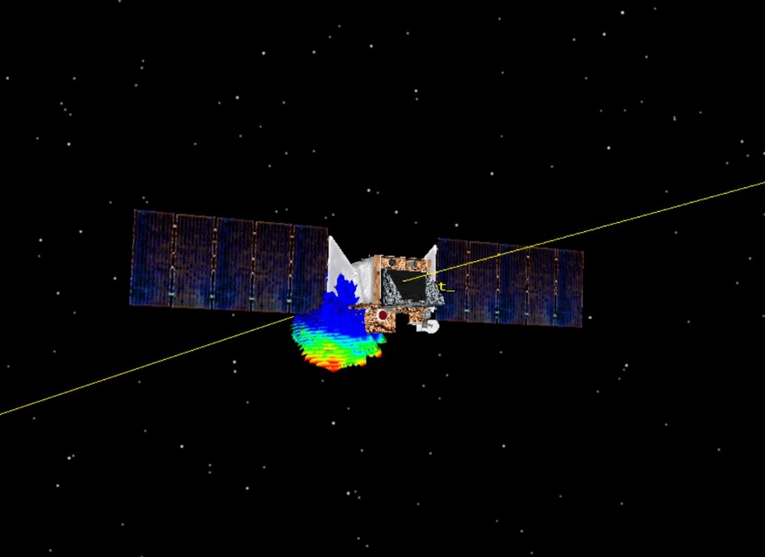
The model is isolated from the model of the satellite. It does not take into account any aspect of the satellite that may affect the signal. The "perfect omni" antenna assumption may not be sufficient for RF link budget modeling.
3D View: Satellite overhead
3D View: Antenna Pattern
Modify the Transmitter
You will analyze the behavior of this system to quantify it in detail. You can model a transmitter to house the antenna and compute the link budget. Transmitter objects can pull in configuration of antennas modeling in the scenario.
- Open Transmitter's () properties ().
- Select the Basic - Definition page.
- Set the Type to Complex Transmitter.
- Click .
- Enter the following Model Specs:
- Click the Antenna tab.
- Set the Reference Type to Link.
- Ensure Antenna/OmniIsolated is set as the Antenna Name.
- Click . The external model has now been imported into STK.
| Option | Value |
|---|---|
| Frequency | 2.2 GHz |
| Antenna Design Frequency | Default |
| Power | 2 W |
| Data Rate | 16 Mb/sec |
There are many default antenna gain patterns available in STK. Instead of these, you can load an external antenna pattern that is relevant to the mission.
Refresh the Link Budget
- Select the Link Budget report.
- Click the Refresh button.
Notice the greater variation in the BER with this updated model. Rather than the constant value, see how the BER varies throughout the satellites pass. This is still an idealized mission model. Realistically the behavior of the antenna changes depending on how it is placed on the body of the satellite. You can analyze that behavior next.
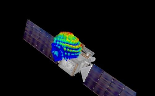
Model the Installed Antenna
To take the satellite model behavior into account, you are using the OmniIsolated file. This file was created using ANSYS HFSS SBR+ that uses Shooting and Bouncing Rays to solve the antenna interaction with the satellite it is attached to. However, the source of the antenna behavior data could come from a multitude of sources. You created your own data in STK, loaded external models, and could have loaded results from system tests.
Antenna performances can be altered dramatically and impact the associated system because of the relationship between vehicle and payload. This is important to take into account in the mission model. This file is the OmniInstalled model because it is takes into account the antenna behavior. Assuming the antenna was installed at a specific location on the body of the vehicle, it would take into account the interference from that location.
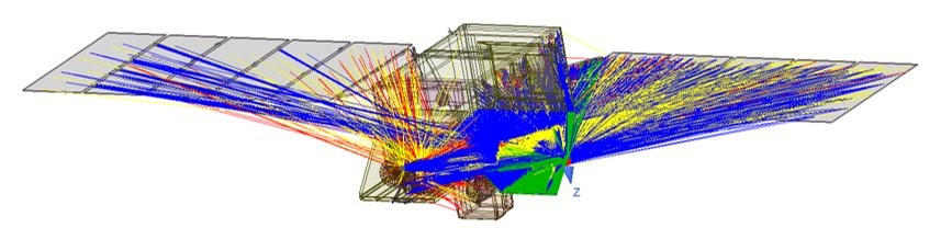
The above figures demonstrate the results from the HFSS SBR+ using Shooting and Bouncing Rays analysis.
- Copy the OmniIsolated antenna ().
- Paste it on LEO_Sat ().
- Rename the antenna OmniInstalled.
- Disable OmniIsolated in the Object Browser.
- Open OmniInstalled's () properties ().
- Select the Basic - Definition page.
- Set the External Filename to SatCom_Omni_2p2G_Installed.pattern.
- Click .
If you were to open the pattern file in a text editor, you'd notice that the values change throughout the file.
Pattern file in Text editor
View in 3D
- Right-click on LEO_Sat () in the Object Browser.
- Select Zoom To.
- Mouse around the 3D Graphics window to understand the new antenna pattern.
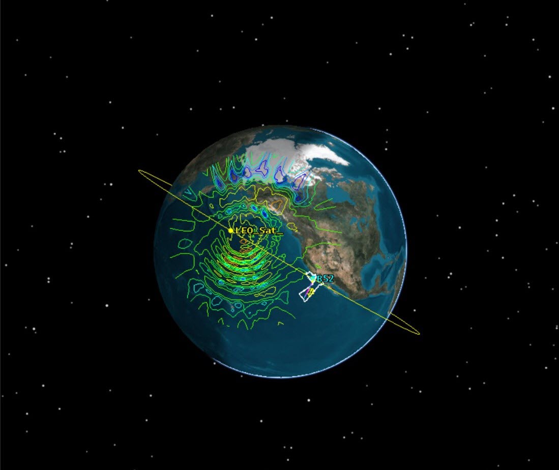
Notice the dramatic difference between the two antenna models. It is also important to understand the affect the interaction of the antenna and satellite can have on the signal. This is visualized with the contours on the surface of the Earth. The effects can also be measured in the data.
Rerun the OmniInstalled Antenna
- Open Transmitter's () properties ().
- Select the Antenna tab.
- Set the Antenna Name to Antenna/OmniInstalled.
- Click .
- Refresh the Link Budget report.
- Save () the scenario.
Examine the data. Notice the dramatic variations in the Bit Error Rate than with the OmniInstalled antenna model. To understand how this antenna model affects the data, you can generate a Bit Error Rate graph.
View in 3D
- Enable the OmniInstalled () antenna in the Object Browser.
- Right-click on LEO_Sat () in the Object Browser.
- Select Zoom To.
- Mouse around the 3D Graphics window to view the contours on the Earth.
- Animate () the scenario.
Over time notice how the pattern of the antenna passes over the Ground Terminal. You can assess this in more detail with a BER graph.
Generate the BER Graph
- Right-click on OmniInstalled () antenna in the Object Browser.
- Select the
 Report & Graph Manager tool.
 - Set the Object Type to Access.
- Expand the Installed Styles directory.
- Generate a Bit Error Rate graph.
- Set the Step Size to one (1) second.
- Draw a box around one of the peaks. This updates the graph to show the data values.
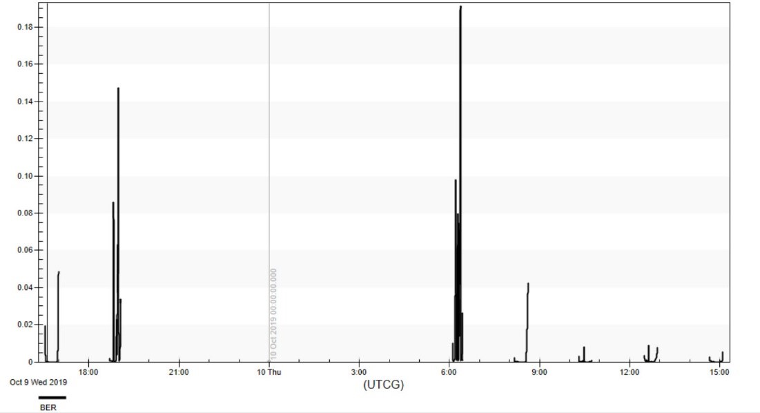
The graph shows the BER throughout the scenario.
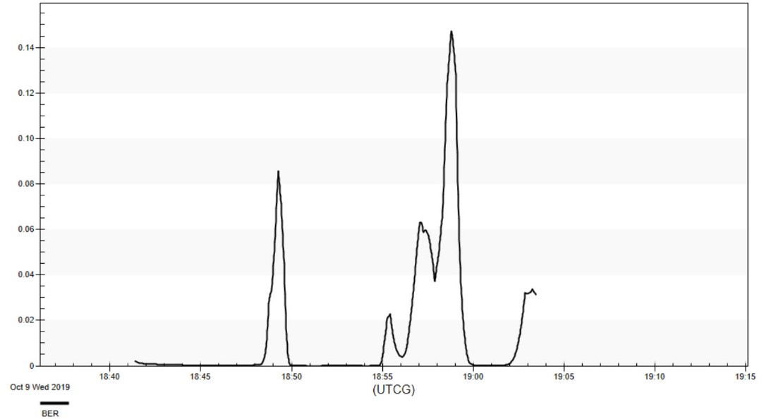
Graph: BER graph
View in 3D
- Right-click on the sharp peak in the graph.
- Select the Set Animation Time option.
- Mouse around in the 3D Graphics window to note the dip in the antenna pattern as it passes over the Ground Terminal.
- Disable the OmniInstalled antenna in the Object Browser.
- Save () the scenario.
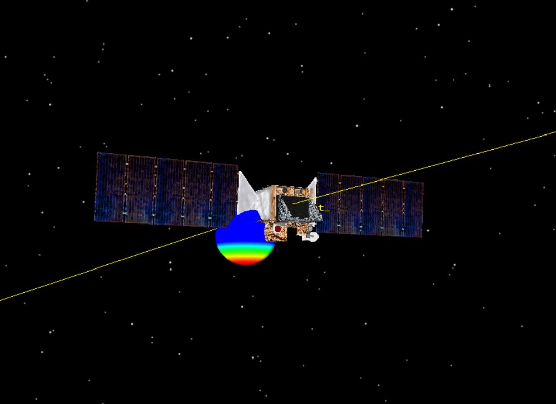
3D View: Antenna Pattern over Ground Terminal
It is important to consider how you would not have known of this loss in signal had you not used a custom external antenna model and generated the BER graph.
Design the Satellite Constellation
- Right-click on LEO_Sat () in the Object Browser.
- Extend the Satellite menu.
- Select the Walker... option.
- Set the following options:
- Click .
- Click Close after all satellites are inserted.
| Option | Value |
|---|---|
| Number of Sats per Plane | 6 |
| Number of Planes | 6 |
| Create Constellation | On |
| Name | LEO_Sats |
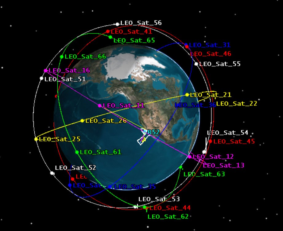
3D View: Walker constellation
Create a Chain Access
The Walker tool allows you to design constellations of satellites using the behavior of a seed satellite. It will also model any payloads on the seed satellite. In this mission that would be the Transmitter & Antennas.
You built a global constellation to provide as much coverage as possible to track the hypersonic vehicle. However, not all of these satellites are overhead during the time of the flight. You only care about a subset of the satellites not all 36 satellites.
To quantify the relationship between all satellites in the constellation and the ground terminal, you can compute a chain access.
- Bring the Insert STK Objects tool () to the front.
- Insert an Chain object (
 ) using the Define Properties () method.
 - Move (
 ) LEO_Sats (
 ) object to the Chain.
 - Move () Ground Terminal ().
- Click .
- Rename the chain LEO_to_Ground.
- Save () the scenario.
You can calculate this analysis with the transmitters. You would need to model the transmitters in a constellation with the receiver. However, in this approach you just want to know when the satellites are overhead of the Ground Terminal.
The Chain access is automatically computed.
Generate Data
- Right-click on Leo_to_Ground () chain in the Object Browser.
- Select the Report & Graph Manager tool.
- Set the Object Type to Chain.
- Expand the Installed Styles directory.
- Generate a Individual Strand Access graph.
- Close the Individual Strand Access graph.
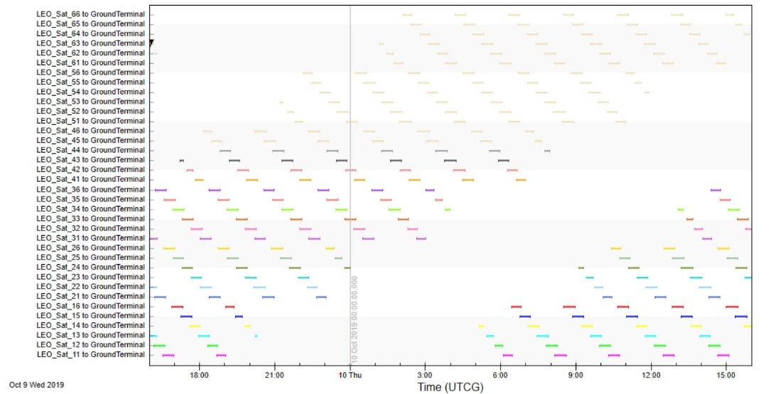
Graph: Individual Strand Access
Define the Custom Intervals
Throughout the period of analysis, you can see all the links between your satellites and the ground terminal. However, you care about how these systems communicate during the period of the X-43's test flight. Let's figure out which satellites are relevant during the flight.
- Set the Time Properties to Specify Time Properties.
- Set the Type to Custom Interval List.
- Click the ellipsis () button.
- Select HXRV_X43 in the STK Object field.
- Select the HXRV_X43 AvailabilityIntervals from the Components List.
- Click .
- Generate the Individual Strand Access graph.
- Save () the scenario.
- Close the scenario.
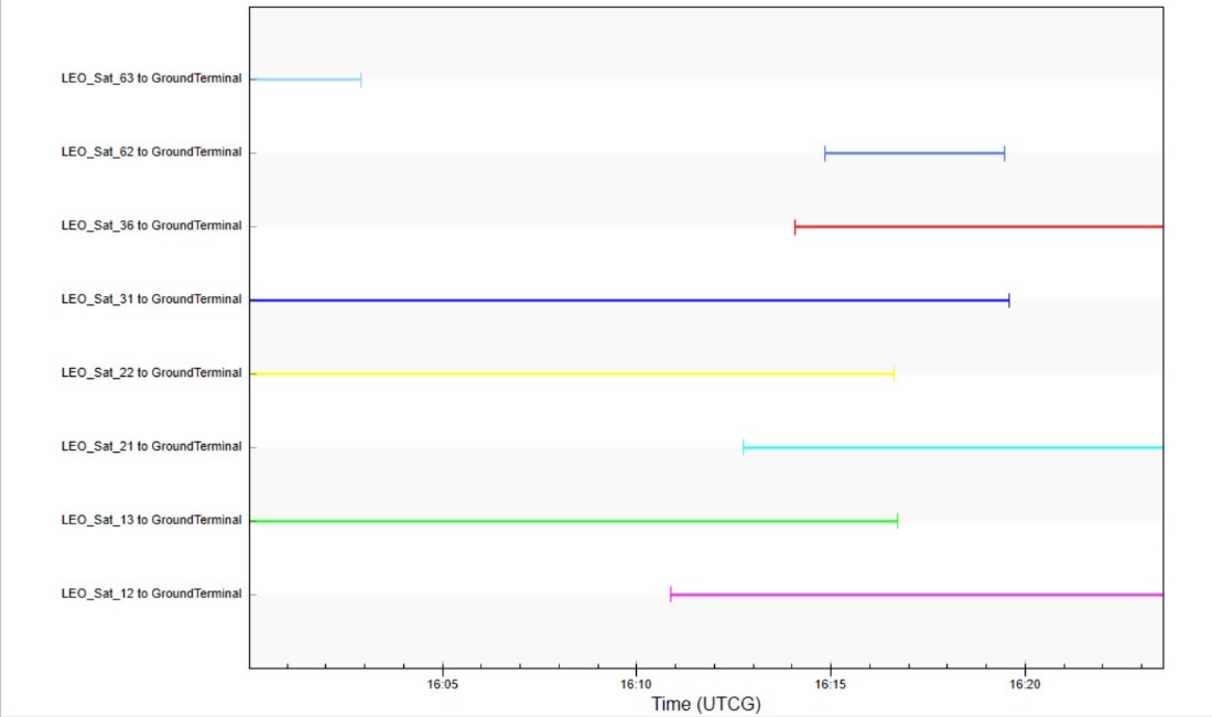
Graph: Modified Individual Strand Access
Now you are just looking at the eight satellites overhead during the time of the flight. Through each stage of the analysis, you needed to reevaluate the outcomes of the mission. Through modifications of the antenna and examining the link budget, you can see the effects through each iteration. This falls directly in line with the DME workflow. Within one system (STK), changing the necessary systems (transmitters) maintain the required mission metrics (Link Budget - BER).
DME: Events and Time Components
In this section, you will focus on understanding and relating all the events that occurred from the beginning of the X43 (HXRV_X43 aircraft object) test flight to when it was tracked and any information relayed. The first session of the 3 part series had us create a unique satellite constellation to track and monitor a hypersonic aircraft. The second session walked us through building the hypersonic flight and comparing it to a model from ANSYS. In that session we also created EOIR synthetic cameras to image the thermal properties of hypersonic. Finally, in the first section of session 3, we created the communication system to covey the message to the necessary systems. This last section of session 3 will bring it all together. We will model how the information will be passed from system to system so the satellites have the opportunity to image the hypersonic aircraft.
Open the Starter Scenario
In this final section of the DME series, you will analyze how all the systems work together. To speed up the analysis, you have a starter scenario to load.
Choose one of the three methods below to open a starter scenario.
Option 1: Open a Starter Scenario From the SDF - Use the Browse Method
If you want to open the starter scenario from the SDF, you can open it by browsing to the VDF file.
- Click the Open a Scenario () button.
- Select STK Data Federate on the left side of the Open window.
- Select the Browse tab.
- Navigate to Sites/AGI/documentLibrary/ STK 12/Starter Tutorials/DME_Session3_Comms_and_Event_Analysis
- Select DME_Session3_Starter_AWB.vdf.
- Click .
Option 2: Open a Starter Scenario From the SDF - Use the URL
If you want to open the starter scenario from the SDF, you can open it by copying and pasting the VDF's URL. The URL is https://sdf.agi.com/share/page/site/AGI/document-details?nodeRef=workspace://SpaceStore/75da1baf-9c8f-4f06-b9d8-98d433a997f3
- Click the Open a Scenario () button.
- Select STK Data Federate on the left side of the Open window.
- Copy the following url: https://sdf.agi.com/share/page/site/AGI/document-details?nodeRef=workspace://SpaceStore/75da1baf-9c8f-4f06-b9d8-98d433a997f3
- Right-click in the File name: field.
- Select Paste.
- Select DME_Session3_Starter_AWB.vdf.
- Click .
Option 3: Open a Starter Scenario Locally
If you want to open the starter scenario from a local file, follow the steps below.
- Click the Open a Scenario () button.
- Ensure STK User is selected on the left side of the Open window.
- Browse to the location of the saved starter scenario.
- Click .
Save Your Scenario
First you want to save your scenario. The way to save your scenario varies slightly depending if you opened the starter scenario from the SDF or from a local file.
Choose the appropriate save method below based on how you opened the starter scenario.
Option 1: Save Your Scenario After Opening It From the SDF
If you opened the starter scenario from the SDF, follow the steps below to save your scenario.
- Click File on the menu bar.
- Select Save As...
- Select STK User on the left side of the Save As window.
- Click Create New Folder icon.
- Name it X43_Mission_AWB.
- Select the X43_Mission_AWB folder.
- Click .
- Ensure the Save as type: is Scenario Files (*.sc).
- Set the File name: to X43_Mission_AWB.sc.
- Click .
Option 2: Save Your Scenario After Opening It From a Local File
If you opened the starter scenario from a local file, follow the steps below to save your scenario.
- Click File on the menu bar.
- Select Save As...
- Select STK User on the left side of the Save As window.
- Click Create New Folder icon.
- Name it X43_Mission_AWB.
- Select the X43_Mission_AWB folder.
- Click .
- Ensure the Save as type: is Scenario Files (*.sc).
- Set the File name: to X43_Mission_AWB.sc.
- Click .
Examine the Scenario
Examine the scenario when it opens.
- You should see the hypersonic test flight (discussed in DME session 2).
- You should see the eight relevant satellites from the SBIRS LEO Constellation (designed in DME session 1 and refined earlier in this session). These satellites are modeling the OmniInstalled transmitters and the Space-Based Infrared System (SBIRS).
- New to the mission are geosynchronous satellites. These satellites are modeling the Defense Support Program (DSP) detection system.
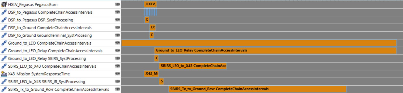
All data and behavior is notional. Here are how the systems relate.
- The mission is initiated by a launch of a B2 carrying the HXLV Pegasus which accelerates the HXRV X43.
- When the Pegasus ignites (begins its burn), it is detectable.
- The DSP satellites in geo-orbit search for rocket plumes (ignition signature).
- When a burn signature (something big and bright) is detected and processed, the DSP system sends that information to a Ground Terminal.
- The Ground Terminal receives the information, processes it, and sends it to a constellation of SBIRS LEO satellites. The basis of this constellation is from Session 1, but with modifications that came about as the mission scope was expanded.
- The satellites have IR cameras on-board to track and follow the X43 once it has been released from the Pegasus.
- That information is transmitted back down to the Ground Terminal.
- Once this entire system is modeled, you can assess the Total System Response Time, from the rocket ignition to full tracking by the SBIRS LEO Satellites.
Add the Pegasus Burn to the Timeline View
The event that triggers the DSP and thus the entire series is the burn from the Pegasus launch. You can add that to the timeline to see when it occurs.
- Select the Add Time Components (
 ) option from the Timeline View.
 - Select the HXLV_Pegasus as the STK Object.
- Select PegasusBurn from the Components List. This component was pre-built in the starter scenario. It has defined start and end time for the duration of the burn.
- Click .
- Save () the scenario.
- Click and drag the markers on either side to resize the timeline.

Pegasus Burn: This ignition burn is the initial event that triggers a detection system. It is what sets off the series of following events
You can use the Timeline View Port markers to focus on smaller periods of the scenario. You need to move forward in time of the scenario to see the rectangular marker on the left.
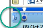
This adds the first-time component to the Timeline. This component was built to model the burn of the Pegasus as it takes off. This is also what the satellites in GEO detecting the burn sees. This is the initial trigger that sets the system in motion. Next, model how well the DSP system can detect the Pegasus.
Create a Chain Between the DSP and Pegasus
Once the Pegasus ignites and takes off, the GEO satellites sweep and look for its signature. You can create a Chain between the system on the GEO satellite (Defense Support Program) to the Pegasus. The sensor is a specific system that is in the correct position to detect the Pegasus. Using a chain object, you can do additional analysis.
- Bring the Insert STK Objects tool () to the front.
- Insert an Chain object () using the Define Properties () method.
- Move () the SBIRS_GEO-3_41937/dsp_sweep3 as the first Assigned Object. This is the specific system that is in the right location to detect the ignition.
- Move () the HXLV_Pegasus as the second Assigned Object.
Define the Interval Component
This models the detection of the burn through each sensor sweep. This sensor is attached to a satellite spinning and sweeping the sensor over the earth. Through each sweep the system is triggered when it detects the burn. You can add the burn interval to the chain analysis to make sure you are looking at it during the correct period.
- Select the Basic - Advanced page.
- Set the Compute Time Period to User Specified Time Period.
- Select Interval Component... from the drop-down.
- Select the HXLV_Pegasus as the STK Object.
- Select PegasusBurn from the Components List.
- Click .
- Click to close the Chain properties.
- Rename the chain object DSP_to_Pegasus.
- Save () the scenario.
Add the Time Component to the Timeline View
You can add the time component to the Timeline View to see how it compares to the data you have about the Pegasus burn.
- Select the Add Time Components () option from the Timeline View.
- Select the DSP_to_Pegasus as the STK Object.
- Select CompleteChainAccessIntervals from the Components List.
- Click .

DSP_to_Pegaus CompleteChainAccessIntervals: This interval marks each time the sensor on the SBIRS_GEO-3_41937 is able to scan and detect the burn signature from the burn
Create System Processing Duration
This component shows all the instances when the DSP on-board the satellite can detect the Pegasus burn. However, the system needs to verify that it is detecting a real ignition and process that information before it can relay it to the ground system. You can build the chain between the DSP to the ground station while taking the processing time into account.
- Open Analysis Workbench (
 ).
). - Ensure the Time tab is selected.
- Select the DSP_to_Pegasus () as the STK Object. You can build the processing time on this chain access.
- Click the Create new Interval (
 ) button.
Create a Time Component
- Set the Type to Fixed Duration.
- Set the component name to DSP_SystProcessing.
- Click the ellipsis () button to change the Reference Time Instant.
- Set the component to DSP_to_Pegasus CompleteChainAccessTimeSpan.Start.
- Set the Stop Offset to 30 sec.
- Click .
- Drag DSP_SystProcessing to the Timeline.
- Close the Analysis Workbench.
This allows you to build the processing time from the first detection of the burn.
You built this component so that it is triggered during the first sweep and after the third one is prepared to relay the information.
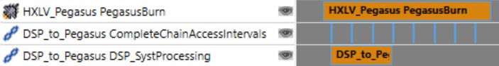
DSP_to_Pegaus DSP_SystProcessing: This interval accounts for how long the information takes to process on-board the SBIRS_GEO-3_41937 and when it is able to react.
Create a Chain Between the DSP to the Ground Terminal
After the burn is verified and the information processed, the next stage is to send that signal to the ground terminal. You do not have a specific transmitter built on this system so the analysis focuses on the chain access between the geostationary satellite and the ground terminal.
- Bring the Insert STK Objects tool () to the front.
- Insert an Chain object () using the Define Properties () method.
- Move () the SBIRS_GEO-3_41937 as the first Assigned Object.
- Move () the GroundTerminal as the second Assigned Object.
- Click Apply.
Define the Interval Component
This models the access between the satellite in geo and the ground terminal. The access begins after the signal has been processed. You set this up in the advanced settings.
- Select the Basic - Advanced page.
- Set the Compute Time Period to User Specified Time Period.
- Expand the Start Time menu from the drop-down.
- Select the Time Component option.
- Select the DSP_to_Pegasus as the STK Object.
- Expand the DSP_SystProcessing component.
- Select Stop. You want the chain access to begin once the information from the geostationary satellite is processed and sent.
- Click .
Define the End of the Chain
You can repeat the same process to set the Stop component. You want to define the end of the chain access.
- Expand the Stop Time menu from the Interval drop-down.
- Select Time Component.
- Select DSP_to_Pegasus as the STK Object.
- Expand the CompleteChainAccessIntervals components.
- Expand the Last component.
- Select Stop.
- Click .
- Click to close the chain properties.
- Rename the chain to DSP_to_Ground.
- Save () the scenario.
Add the Component to the Timeline View
- Select the Add Time Components () option from the Timeline View.
- Select the DSP_to_Ground as the STK Object.
- Select CompleteChainAccessIntervals from the Components List.
- Click .
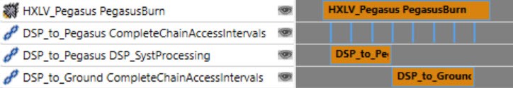
DSP_to_Ground CompleteChainAccessIntervals: The interval added to the timeline accounts for when the SBIRS_GEO-3_41937 is able to send information down to the Ground Terminal.
Ground Terminal Processing Time
Once the Ground Terminal has the message from the Defense Support System, it processes and relays the message to the SBIRS LEO constellation. You can build that component next.
- Open Analysis Workbench ().
- Ensure the Time tab is selected.
- Select the DSP_to_Ground () as the STK Object. You can build the processing time on this chain access.
- Click the Create new Interval () button.
Create a Time Component
- Set the Type to Fixed Duration.
- Set the component name to GroundTerminal_SystProcessing.
- Set the Stop Offset to 30 sec.
- Click .
- Drag GroundTerminal_SystProcessing to the Timeline.
- Close the Analysis Workbench.
- Save () the scenario.
This component accounts for the processing time at the Ground Terminal before it relays the message.
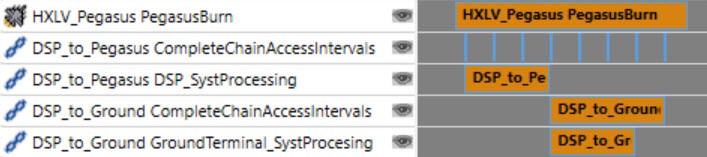
DSP_to_Ground GrountTerminal_SystemProcessing: The Ground Terminal processes the information it receives from the SBIRS_GEO-3_41937. Once processed it can share it.
Create a Chain Between Ground Terminal to SBIRS LEO Satellites
The Ground Terminal relays the message to the constellation of SBIRS LEO satellites. It doesn't matter what satellites get the message. You can send the message to any satellite overhead.
- Bring the Insert STK Objects tool () to the front.
- Insert an Chain object () using the Define Properties () method.
- Move () the GroundTerminal as the first Assigned Object.
- Move () the SBIRS_LEO as the second Assigned Object.
- Click .
- Rename the chain object Ground_to_LEO.
- Save () the scenario.
Define the Interval
Add the time component to the Timeline to see how it relates to the intial stages of the mission.
- Select the Add Time Components () option from the Timeline View.
- Select the Ground_to_LEO as the STK Object.
- Select CompleteChainAccessIntervals from the Components List.
- Click OK.
You confirmed that you can see this interval throughout the length of the mission. Now you can create a component that looks at just when the signal is transmitted.
Create a Chain from Ground Terminal to SBIRS LEO When the Message is Relayed
This chain is similar to the previously built component, however, this time you can view the chain link after the signal is sent from the Ground Terminal until the end of the previously built chain access.
- Bring the Insert STK Objects tool () to the front.
- Insert an Chain object () using the Define Properties () method.
- Move () the GroundTerminal as the first Assigned Object.
- Move () the SBIRS_LEO as the second Assigned Object.
- Click .
- Rename the chain object Ground_to_LEORelay.
- Save () the scenario.
Specify the Start Time Component
- Select the Basic - Advanced page.
- Set the Compute Time Period to User Specified Time Period.
- Expand the Start Time menu from the drop-down.
- Select the Time Component option.
- Select the DSP_to_Ground () as the STK Object.
- Expand the GroundTerminal_SystProcessing component.
- Select Stop. You want the chain access to begin once the information from the Ground Terminal is processed and sent.
- Click OK.
Specify the Stop Time Component
- Expand the Stop Time menu from the drop-down.
- Select the Time Component option.
- Select the Ground_to_LEO as the STK Object.
- Expand the CompletedChainAccessTimeSpan component.
- Select Stop. This access takes place once the message is sent from the Ground Terminal until the satellites are no longer in view.
- Click .
- Click to close the chain properties.
- Save () the scenario.
Add the Time Component to the Timeline View
- Select the Add Time Components () option from the Timeline View.
- Select the Ground_to_LEORelay as the STK Object.
- Select CompleteChainAccessIntervals from the Components List.
- Click .
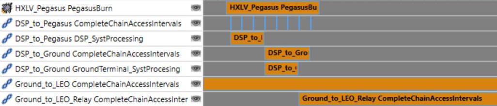
Ground_to_LEO_Relay CompleteChainAccessIntervals: This interval shows how long the Ground Terminal has to relay information to the constellation of LEO satellites.
Create SBIRS System Processing Time
- Open Analysis Workbench ().
- Ensure the Time tab is selected.
- Select the Ground_to_LEORelay () as the STK Object. You can build the processing time on this chain access.
- Click the Create new Interval () button.
Create a Time Component
- Set the Type to Fixed Duration.
- Set the component name to SBIRS_SystProcessing.
- Set the Stop Offset to 30 sec.
- Click .
- Drag SBIRS_SystProcessing to the Timeline.
- Close the Analysis Workbench.
- Save () the scenario.
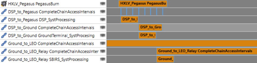
Ground_to_LEO_Relay SBIRS_SystProcessing: The LEO constellation isn’t able to react immediately, this interval accounts for how long it takes for it to take action.
Create a Chain from the SBIRS LEO to the X43
Now that you know how long it takes the transmitters to react, you can create a chain access between the SBIRS LEO constellation and the X43.
Once the SBIRS LEO system knows the Pegasus launch has taken place, it can lock on and begin to track the rest of the X43 flight.
- Bring the Insert STK Objects tool () to the front.
- Insert an Chain object () using the Define Properties () method.
- Move () the SBIRS_LEO as the first Assigned Object.
- Move () the HXRV_X43 as the second Assigned Object.
- Click Apply.
- Rename the chain object SBIRS_LEO_to_X43.
- Save () the scenario.
This models the access between the SBIRS_LEO system and the rest of the X43 test flight. You are going to account for how long it takes for the SBIRS system to react to the message from the Ground Terminal.
Specify the Start Time Component
- Select the Basic - Advanced page.
- Set the Compute Time Period to User Specified Time Period.
- Expand the Start Time menu from the drop-down.
- Select the Time Component option.
- Select the Ground_to_LEORelay as the STK Object.
- Expand Select SIRBS_SystProcessing.
- Select Stop.
Specify the Stop Time Component
- Expand the Stop Time menu from the drop-down.
- Select the Time Component option.
- Select the HXRV_X43 as the STK Object.
- Expand the AvailablityTimeSpan component.
- Select Stop. This access takes place once the message is sent from the Ground Terminal until the satellites are no longer in view.
- Click .
- Click to close the chain properties.
- Save () the scenario.
Add the Time Component to the Timeline View
- Select the Add Time Components () option from the Timeline View.
- Select the SBIRS_LEO_to_X43 as the STK Object.
- Select CompleteChainAccessIntervals from the Components List.
- Click .
- Save () the scenario.
Examine the Total System Response Time
You can now see how long it takes from the initial launch to when the SBIRS system can track the rest of the X-43 flight. You can measure this explicitly.
From the beginning of the DSP’s detection of the Pegasus launch to when the SBIRS system locks on is the total system response time. You can build this component in STK's Analysis Workbench capability.
- Open Analysis Workbench ().
- Ensure the Time tab is selected.
- Select the X43_Mission_AWB (
 ) as the STK Object. You can build the processing time on this chain access.
 - Click the Create new Interval () button.
Create a Between Instants Component
- Set the Type to Between Time Instants
- Set the component name to SystemResponseTime.
- Set the Start Time Instant to HXLV_Pegasus PegasusBurn Start.
- Set the Stop Time Instant to SBIRS_LEO_to_X43 CompleteChainAccessTimeSpan Start.
- Click .
- Click .
- Drag SystemResponseTime to the Timeline.
- Close the Analysis Workbench.
- Save () the scenario.
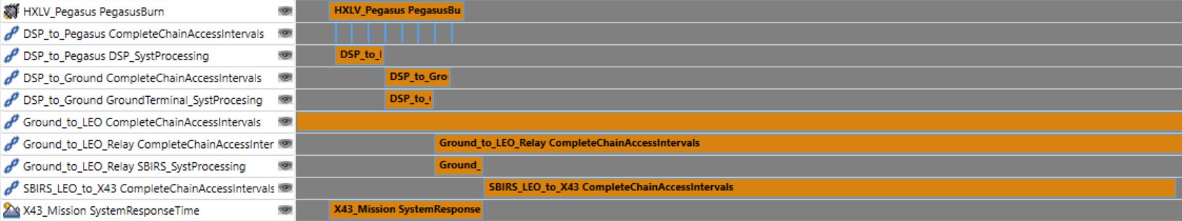
X43_Mission SystemResponseTime: This is how long it would take for a space based system to know that a hypersonic vehicle has been launched. From the initial burn, to when the LEO constellation is informed of the launch is the System Response Time.
Examine the timeline. The newly added component is the full closed loop of a system response. If you hover over the SystemResponseTime interval, you can see the total duration.
SBIRS LEO IR Tracking and Processing
You can complete the system. The SBIRS LEO constellation has an IR Tracking system on it. It tracks the X43, processes it, and sends the information back to the Ground Terminal Receiver.
- Open Analysis Workbench ().
- Ensure the Time tab is selected.
- Select the SBIRS_LEO_to_X43 () as the STK Object. You can build the processing time on this chain access.
- Click the Create new Interval () button.
Create a Time Component
- Set the Type to Fixed Duration.
- Set the component name to SBIRS_IR_SystProcessing.
- Set the Stop Offset to 30 sec.
- Click .
- Drag SBIRS_IR_SystProcessing to the Timeline.
- Close the Analysis Workbench.
- Compute the SBIRS_LEO_to_x43 () access.
- Save () the scenario.
Create a Chain to Model the Communication Link
- Bring the Insert STK Objects tool () to the front.
- Insert an Chain object () using the Define Properties () method.
- Move () the SBIRS_LEO_Tx as the first Assigned Object.
- Move () the Ground as the second Assigned Object. This models the communication link between the transmitters on the satellites and the receiver on the ground. You also want to take into account the time for the signal to process.
- Click Apply.
- Rename the chain object SBIRS_Tx_to_Ground_Rcvr.
- Save () the scenario.
Specify the Start Time Component
- Select the Basic - Advanced page.
- Set the Compute Time Period to User Specified Time Period.
- Expand the Start Time menu from the drop-down.
- Select the Time Component option.
- Select the SBIRS_LEO_to_X43 as the STK Object.
- Expand the SBIRS_IR_SystProcessing component.
- Select Stop. You want the chain access to begin once the information is processed.
- Click .
Specify the Stop Time Component
- Expand the Stop Time menu from the drop-down.
- Select the Time Component option.
- Select the Ground_to_LEO as the STK Object.
- Expand the CompleteChainAccessTimeSpan component.
- Select Stop. You already measured the inter-visibility between the SBIRS satellites and the Ground Terminal. The end time of this component works for the link.
- Click .
- Disable the Automatically Recompute Access option. This chain is dependent on many earlier chains. When you make changes to the study, you want to manually update this calculation so it takes the latest configuration.
- Click to close the chain properties.
- Right-click on the SBIRS_Tx_to_Ground_Rcvr () Chain in the Object Browser.
- Select Chain to open the Chain menu.
- Select Compute Accesses.
- Save () the scenario.
Add the Time Component to the Timeline View
- Select the Add Time Components () option from the Timeline View.
- Select the SBIRS_Tx_to_Ground_Rcvr as the STK Object.
- Select CompleteChainAccessIntervals from the Components List.
- Click OK.
- Save () the scenario.
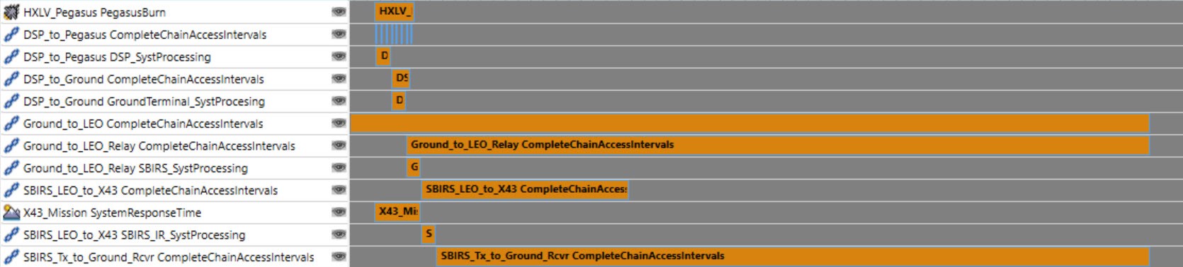
SBIRS_Tx_to_Ground_Rcvr CompleteChainAccessIntervals: The LEO constellation is equipped with IR cameras. It will transmit that data back down to the Ground Terminal.
Take a look at the timeline. You can see the total system of systems working together, sending information, relaying it, and processing it. This provides you with a holistic view of the mission design. You can also analyze what happens when events go awry.
Digital Thread Analysis - Losing Satellites
The basis of our constellation is that it will provide us with persistent coverage with at least two satellites covering our region. That means, even if two satellites get knocked out, we will still be able to track out X43. Let’s test this out.
- Open SBIRS_LEO () properties ().
- Remove (
 ) the SBIRS_LEO12 () from the list of Assigned Objects.
 - Click OK.
- Open Ground_to_LEO's () properties ().
- Select the Basic - Advanced page.
- Disable the Automatic Recompute Accesses option.
- Click OK.
- Right-click on Ground_to_LEO ().
- Extend the Chain menu.
- Select the Compute Access option.
- Recompute the other dependent chains:
- Ground_to_LEORelay
- SBIRS_LEO_to_X43
- SBIRS_Tx_to_Ground_Rcvr
Lose Three Satellites
- Open SBIRS_LEO's () properties ().
- Remove () the following satellites from the Assigned Objects list:
- SBIRS_LEO21
- SBIRS_LEO36
- Click Apply.
- Right-click on Ground_to_LEO ().
- Extend the Chain menu.
- Select the Compute Access option.
- Recompute the other dependent chains:
- Ground_to_LEORelay
- SBIRS_LEO_to_X43
- SBIRS_Tx_to_Ground_Rcvr
There is no change in the SBIRS_LEO_to_X43's ability to track the X43. The Ground_to_LEO has become shorter.
Lose Four Satellites
- Bring SBIRS_LEO's () properties () to the front.
- Remove () the SBIRS_LEO62 () from the list of Assigned Objects.
- Click Apply.
- Right-click on Ground_to_LEO ().
- Extend the Chain menu.
- Select the Compute Access option.
- Recompute the other dependent chains:
- Ground_to_LEORelay
- SBIRS_LEO_to_X43
- SBIRS_Tx_to_Ground_Rcvr
Now the SBIRS_LEO_to_X43's ability to track the X43 is shorter. You are no longer able to track the X43 at the end of the flight.
Add the Satellites Back into System
You have the benefit of designing a system specifically to track launches, so the persistent coverage is very good. Even if you lose three satellites, you are able to track the objects. It’s once you lose that fourth satellite that you run into gaps in your data.
- Bring SBIRS_LEO's () properties () to the front.
- Add () the following satellites back into the constellation:
- SBIRS_LEO12
- SBIRS_LEO21
- SBIRS_LEO36
- SBIRS_LEO62
- Click to accept the properties.
- Recompute the other dependent chains:
- Ground_to_LEORelay
- SBIRS_LEO_to_X43
- SBIRS_Tx_to_Ground_Rcvr
- Save () the scenario.
You could also understand this behavior by generating an Individual Strand Access graph on the Ground_to_LEO chain. This graph gives a visual display of which satellites are overhead and when.
Digital Thread Analysis - Communications Link BER
You can also stress test the communication link that is relaying the message back down to the ground terminal. Earlier we discussed the BER and how it could affect the information transmitted. You can incorporate a constraint on the BER and the constraints of the study. For this mission the easiest way to do that is to set a constraint on the receiver object. Then you can place all the transmitters in a constellation, create a chain access, and generate a link budget on the chain.
The final stage of this mission is a communication link between the SBIRS LEO transmitters and the Ground terminal receiver. You know that the data will get worse with a higher BER and so you can add a constraint to the mission model that takes into account when you have bad data.
- Open SatCommRcvr's () properties ().
- Select the Constraints - Comm page.
- Enable the Bit Error Rate - Max constraint.
- Set the Max value to 1e-09.
- Click .
- Recompute the SBIRS_Tx_to_Ground_Rcvr () object.
- Save () the scenario.
Note how the BER constraint means that data transmitted at the beginning and end of the link is no longer valid. The total time to send the IR information is cut down.
SBIRS_Tx_to_Ground_Rcvr CompleteChainAccessIntervals: Examine the beginning and end of the interval, it is much shorter due to the constraint. With the BER constraint we can see how we will lose the ability to transmit data to the Ground Terminal. The duration of the access interval is much shorter, not because the satellites aren’t there, but because the data quality is worse.
The purpose of this series and of this mission is to evaluate how all the components of the mission work together. In previous sessions, you built detailed models, and in this scenario were able to bring them all together to see how they affect one another. You can evaluate your mission’s outcomes through an integrated digital environment, STK.