STK Premium (Air), or STK Enterprise
You can obtain the necessary licenses for this training by contacting AGI Support at support@agi.com or 1-800-924-7244.
Additional installation - EOIR. You can obtain the necessary install by visiting http://support.agi.com/downloads or calling AGI support.
The results of the tutorial may vary depending on the user settings and data enabled (online operations, terrain server, dynamic Earth data, etc.). It is acceptable to have different results.
If you have not completed Part 1 of the DME lessons, a starter scenario is provided. It requires STK 12 or newer to open. The DME lessons are in the Training - Level 3 - Focused tutorials section of the STK Help.
Capabilities Covered
This lesson covers the following STK Capabilities:
- STK Pro
- Aviator
- Aviator Pro
- Analysis Workbench
- Electro-Optical Infrared Sensor Performance (EOIR)
Problem Statement
Across the industry, the digital engineering process is becoming more complex. Systems of systems are changing and updating in different stages of the mission lifecycle. In this series, we will address these challenges by creating a fully connected digital thread with a common mission environment at the core. We will design and test a new satellite constellation for persistent, stereo coverage of hypersonic vehicles across the world. We will discuss this topic in stages: satellite constellations, hypersonic flight, EOIR synthetic sensors, communications links, and triggering events and systems. Our vision is to integrate the mission environment and operational objectives into the digital thread early and throughout the entire product lifecycle. Through digital mission engineering, we are now capable of quickly evaluating the overall mission impact of the smallest change to any component. This session will advance to the detailed engineering phases where we will demonstrate how to incorporate higher fidelity third party models of sensors and vehicle heat signatures into the mission model and understand the respective analytical results.
Solution
In this section of the DME series, we will focus on using externally created CFD results to populate the performance model of an aircraft and the thermal signature for use with STK's Aviator and EOIR capabilities.
We will recreate NASA's 2004 X-43 Hypersonic test flight path using our ANSYS Fluent generated performance characteristics. We will also incorporate test range assets and evaluate how well they should be able to monitor the flight based on the thermal signature also provided by the CFD analysis.
The original X-43 test was composed of several procedures that we will include in our Aviator mission. The mission begins with a B52 carrying the combined launch vehicle and hypersonic test vehicle. The B52 takes off from Pt. Mugu and flies out out to the Pacific Test Range. Once the B52 has entered the test region, it releases the modified Pegasus launch vehicle known as the Hyper X Launch Vehicle (HXLV). This launch vehicle accelerates the X-43 Hyper X Research Vehicle (HXRV) to Mach The ratio of the aircraft's speed and the speed of sound at the aircraft's altitude, with local atmospheric conditions. 9 and an altitude of 110,000 ft before separating. At that point, the X-43 conducts a short test of the scramjet to maintain velocity before finally gliding down to the sea. We will use the lift and drag coefficients found with CFD to define how the vehicle behaves over the flight envelope.
Once we've modeled the flight path, we will switch our focus to evaluating various sensor responses with EOIR based on the thermal signature, again from our CFD runs. This will tell us how well our test assets will be able to monitor the test mission as it progresses.
Upon completion of this tutorial, you will be able to create the following:
- Experience building new vehicle profiles in STK's Aviator Pro capability.
- Design a flight in Aviator.
- Practice comparing results at varying levels of fidelity.
- Build an EOIR sensor and tracking an object.
- Gain experience loading in external files from other tools.
External Files
- DME_Session2_Starter_Aviator_EOIR.vdf - This is the starter scenario for this lesson.
- X-43.mdl - This is the custom aircraft model.
- X-43_ANSYS_CFD.aero - This is an external file generated by AGI with ANSYS tools of the hypersonic vehicle's computational fluid dynamics
- x-43_eoir_v03.obj - This is a thermal model for the hypersonic vehicle.
The external files are available for download from the STK Data Federate, AGI - Document Library- STK 12 - Starter Tutorials - DME_Session2_Hypersonics and EOIR in the Operational Environment
Video Guidance
Watch the following video. Then follow the steps below, which incorporate the systems and missions you work on (sample inputs provided).
Open a Starter Scenario
We built a starter scenario for you that contains the flight and the Pegasus hypersonic vehicle. You can open the scenario from the SDF or from the local copy you downloaded from the SDF.
Choose one of the three methods below to open a starter scenario.
Sign in to access the SDF
You can access your scenarios or objects from the STK Data Federate (SDF).
- Click (
 ) in the Welcome to STK dialog box.
 - Change the Location: to STK Data Federate at the bottom of the Open dialog window.
- Click Guest in the top right corner to sign into your account.
- Click when the SDF Server Login dialog box opens.
- Enter your Account name and Password on the Log In: AGI SEDS dialog box.
- Click .
Option 1: Open a Starter Scenario from the SDF - Use the Browse Method
If you want to open the starter scenario from the SDF, you can open it by browsing to the VDF file.
- Select the Browse tab.
- Navigate to Sites/AGI/documentLibrary/ STK 12/Starter Tutorials/DME_Session2_Hypersonics and EOIR in the Operational Environment.
- Select DME_Session2_Starter_Aviator_EOIR.vdf.
- Click .
When the scenario loads, ensure the HXLV_Pegasus aircraft is in the scenario. The aircraft contains the notional aerodynamics model from ANSYS.
Option 2: Open a Starter Scenario Using the URL
If you want to open the starter scenario from the SDF, you can open it by copying and pasting the VDF's URL. The URL is https://sdf.agi.com/share/page/site/AGI/document-details?nodeRef=workspace://SpaceStore/d3668deb-fdc1-419f-ad26-b22d46422859
- Copy the following url: https://sdf.agi.com/share/page/site/AGI/document-details?nodeRef=workspace://SpaceStore/d3668deb-fdc1-419f-ad26-b22d46422859
- Right-click in the File name: field.
- Select Paste.
- Select DME_Session2_Starter_Aviator_EOIR.vdf.
- Click .
When the scenario loads, ensure the HXLV_Pegasus aircraft is in the scenario. The aircraft contains the notional aerodynamics model from ANSYS.
Save Your Scenario
First you want to save your scenario. The way to save your scenario varies slightly depending if you opened the starter scenario from the SDF or from a local file.
Choose the appropriate save method below based on how you opened the starter scenario.
Option 1: Save Your Scenario After Opening It From the SDF
If you opened the starter scenario from the SDF, follow the steps below to save your scenario.
- Click File on the menu bar.
- Select Save As...
- Select STK User on the left side of the Save As window.
- Select DME_Session2_Starter_Aviator_EOIR folder.
- Click .
- Change Save as type: to Scenario Files (*.sc).
- Ensure the File name is DME_Session2_Starter_Aviator_EOIR.sc.
- Click .
- Click . to replace the existing file.
Option 2: Save Your Scenario After Opening It From a Local File
If you opened the starter scenario from a local file, follow the steps below to save your scenario.
- Click File on the menu bar.
- Select Save As...
- Select STK User on the left side of the Save As window.
- Click Create New Folder icon.
- Name it DME_Session2_Starter_Aviator_EOIR.
- Select the DME_Session2_Starter_Aviator_EOIR folder.
- Click .
- Ensure the Save as type: is Scenario Files (*.sc).
- Set the File name: to DME_Session2_Starter_Aviator_EOIR.sc.
- Click .
Insert an aircraft
You can model the hypersonic vehicle by using an aircraft object.
- Bring the Insert STK Objects tool (
 ) to the front.
 - Insert an Aircraft object (
 ) using the Define Properties (
 ) method.
 - Set the Propagator to Aviator.
- Click the Select Aircraft (
 ) button.
 - Right-click on User Missile Models.
- Select New Item.
- Rename the New Missile X-43.
- Click .
- Click .
Flight Path Warning
Aviator performs best in the 3D Graphics window when the surface reference of the globe is set to Mean Sea Level. You will receive a warning message when you apply changes or click OK to close the properties window of an Aviator object with the surface reference set to WGS84. It is highly recommended that you set the surface reference as indicated before working with Aviator.
- When the Flight Path Warning window opens, click the button.
- Click .
The reason we are using the Missile Model is this is a unique Hypersonic Vehicle in that it is mainly a Gliding Hypersonic Vehicle. Depending on the application, you may want to model the hypersonic vehicle as an aircraft.
Hypersonic Properties
You can begin by designing the hypersonic vehicle. You can begin by defining the performance models by assigning the upper limit to the altitude and speed of the vehicle. The vehicle flies around 100,000 feet, but may raise a bit above that value. The value just provides a tolerance value. The same can be said about the Mach number. Even though this aircraft flies at Mach 10, it is closer to Mach 9.6-9.7.
- Click the Aircraft Properties (
 ) button.
 - Ensure the Performance Models tab is selected.
Level Turns
- Locate the Level Turns field.
- Set the Max Load Factor to 15 G-SeaLevel.
- Select Scale by Atmosphere density from the drop-down.
Cruise
- Locate the Cruise field.
- Set the Max Airspeed to Mach 10.
- Set the Default Cruise Altitude to 110000 ft.
Descent
- Locate the Descent field.
- Set the Airspeed to Mach 10.
3D Model
- Locate the model field.
- Click the ellipsis (
 ) button to navigate to the location of x-43 model file. If the file has not been downloaded, it can be searched and loaded in from the STK Data Federate.
 - Select x-43.mdl.
- Click Open.
- Click .
Aerodynamic Properties
You can set the aerodynamics properties of the aircraft. The values were disclosed in the public NASA papers and schematics on the x-43.
- Select the Aerodynamics tab.
- Set the following options:
- Click .
| Option | Value |
|---|---|
| Reference Surface Area | 43 ft^2 (3.99483 m^2) |
| Cl Max | 0.085 |
| Cd | 0.015 |
| Calculate AOA | On |
| Max AOA | 20 deg |
The angle of attack The angle between the body X axis and the projection of the velocity vector onto the body XZ plane. The velocity vector is the velocity of the object as observed in the object's central body fixed coordinate system. change is to add tolerance. It is the max AOA based on certain Cl curves that were made publicly available.
Propulsion tab
You won't make any changes to the propulsion tab, but take a look at the settings.
- Click the Propulsion tab.
- Review the settings.
- Click .
Thermal tab
STK v12.1 or newer provides new thermal performance models to support the design and operations of hypersonic vehicles and related defensive systems. These models, based on the NASA TFAWS analysis, employ a variety of techniques to determine heat flux, heat load, and wall temperatures for any Aviator trajectory. These new thermal performance models can also interface directly with Computational Fluid Dynamics (CFD) models. This is key for both vehicle design, and the analysis of offensive and defensive systems and tactics, where aerodynamic heating plays a significant role in the vehicle signature.
- Click the Thermal tab.
- Review the settings. The Strategy being used is a Basic Thermal model using the Sutton Graves Heat Flux. Users with their own model can plug it in here.
- Modify the Heat Flux Model Params - Leading Radius, set the value to 1 cm (0.01 m). This will model a sharp leading edge.
- Click .
- Click .
Mission Window
You have defined the performance model, but before you start designing the flight, let's update the mission window. The Mission Window is used to define the aircraft's route when Aviator has been selected as the propagator. You want to know what the Mach number throughout the flights. Let's add that next.
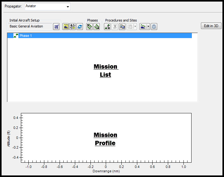
Mission Window
- Right-click on the Mission Profile Window.
- Select Profile Options/Properties.
- Enable the Secondary Y Axis.
- Click on Mach # to select it.
- Click .
- Click .
The Mission Profile Window now displays an additional Y-axis.
Design the X-43 Flight
You created the flight profile and can begin designing the flight. This test flight involved a B52 carrying a modified Pegasus rocket with the X-43 strapped to the front. Due to this, there are a few settings that you need to set to recreate this mission.
The first part is to attach the modified Pegasus Launch Vehicle. During the test it was referred to as the Hyper X Launch Vehicle (HXLV).
- Right-click on Phase 1.
- Select the Insert First Procedure for Phase (
 ) button.
 - Allow the Calculation Progress to finish.
- Select the STK Vehicle site.
- Select the HXLV_Pegasus in the Link To field.
- Click .
Set a Vector Geometry Tool point
- Select
 VGT point.
 - Set the following:
- Click the ellipsis () button beside Formation Point.
- In the Formation Point section, select the HXLV_Pegasus HXRV_X43_LaunchLocation in the Select Position Point window. This is custom point off the body of the vehicle.
- Click to close the Select Position Point window.
| Option | Value |
|---|---|
| Name | AttachedToHXLV |
| Start Time | 1.000 EpSec |
The one second is due to Aviator's interpolation. Aviator needs at least 0.5 seconds of simulation time.
Set the Duration
- Set the Duration to 1500 sec (0.416667 hr).
- Enable the Use Max PointStopTime (no error if <= Duration) option.
- Set the Fuel Flow Source to Override.
- Set the Override Fuel Flow to zero (0) lb/hr. This number is because it is attached to the vehicle.
- Set the Flight Mode to Forward Flight - Cruise.
- Set the Display Step Time to 0.1 sec.
- Click .
By default, Aviator attempts to expend the fuel even if this object is attached. During the test, the X-43 only expended its fuel during the time it was at approximately Mach 10 while attempting to maintain the Hypersonic speed that was achieved by the HXLV.
Set the custom time
- Double-click on Start: 1.000 in the procedure.
- Enable the Set Interrupt Time option.
- Select Time Component from the drop-down.
- Select HXLV_Pegasus in the left column and DeployFromPegasus from Time Instants. This is a custom time to model the aircraft's attachment. This is to model the approximate time at which the charges were set off that released the X-43 from the HXLV.
- Click in the Select Time Instance window.
- Click in the AttachedToHXLV Time window.
- Click .
- Save (
 ) the scenario.
Ejection procedure
Within Aviator there isn't a direct way of modeling an ejection of one aircraft from another. Instead you can represent this stage with a duration of 2.5 seconds of ejection time.
- Right-click on the STK Vehicle Site.
- Select the Insert Procedure After () button.
- Select the End of Previous Procedure (
 ) button.
 - Click .
Define the Ejection Maneuver
- Select the Basic Maneuver (
 ) option.
 - Set the name to Ejection.
- Set the Basic Stop Conditions Time of Flight to 00:00:02.500 HMS.
- Disable the following options:
- Fuel State
- Downrange
- Ensure the Strategy is set to Straight Ahead.
Define the Vertical/Profile
- Select the Vertical/Profile tab.
- Set the following options:
- Locate the Control Limits section.
- Select Specify Max Pitch Rate from the drop-down.
- Set the following options:
| Option | Value |
|---|---|
| Strategy | Autopilot - Vertical Plane |
| Mode | Specify Altitude Change |
| Relative Altitude Change | 100 ft |
| Control Altitude Rate | 2400 ft/min |
| Option | Value |
|---|---|
| Specify Max Pitch | 10 deg/sec |
| Damping Ratio | 2 |
| Airspeed | Maintain current airspeed |
| Maintain Airspeed type | TAS True Airspeed: the speed that the aircraft is moving relative to the airmass that it is flying in. |
Define the Attitude, Performance, and Fuel
- Select the Attitude/Performance/Fuel tab.
- Set the Fuel Flow Source to Override.
- Set the Override Fuel Flow to zero (0) lb/hr. The X-43 at this point is ejected via a release controller on the Pegasus.
- Click .
- Click .
- Save () the scenario.
Fuel Off Performance PreScram
This is the phase where you can model the PreScram measurement phase of the x-43. This is when the vehicle took in data for approximately three (3) seconds before beginning the actual hypersonic gliding process.
- Right-click on the Ejection procedure.
- Select the Insert Procedure After () button.
- Select the End of Previous Procedure () button.
- Click .
Define the Fuel Off Performance PreScram Maneuver
- Select the Basic Maneuver () option.
- Set the name to Fuel Off Performance PreScram.
- Set the Basic Stop Conditions Time of Flight to 00:00:03.000 HMS.
- Disable the following options:
- Fuel State
- Downrange
Define the Navigation Direction
- Set the following options in the Horizontal/Navigation tab:
- Set the Airspeed to Maintain current airspeed.
| Option | Value |
|---|---|
| Strategy | Fly AOA |
| Roll | No Roll |
| AOA | 6 deg |
From the public data, the X-43 maintained an AOA of six (6) degrees, which you just modeled.
Define the Attitude, Performance, and Fuel
- Select the Attitude/Performance/Fuel tab.
- Set the Flight Mode to Forward Flight - Cruise.
- Set the Fuel Flow Source to Override.
- Set the Override Fuel Flow to zero (0) lb/hr. It is a glider and currently using Pegasus' energy.
- Click .
- Click .
- Save () the scenario.
Hypersonic Phase
- Right-click on the Fuel Off Performance PreScram.
- Select the Insert Procedure After () button.
- Select the End of Previous Procedure () button.
- Click .
Define the Hypersonic Maneuver
- Select the Basic Maneuver () option.
- Set the name to Hypersonic.
- Set the Basic Stop Conditions Time of Flight to 00:00:11.000 HMS.
- Disable the following options:
- Fuel State
- Downrange
The vehicle doesn't technically use fuel unless it is in the hypersonic phase. It cannot get to hypersonic, only maintain and glide. This is where you are burning all the fuel the hypersonic vehicle has within it to maintain the hypersonic speed the HXLV has brought to it. You can set the throttle to 100% because there was no throttling on the glider to control this.
Define the Navigation Direction
- Set the following options in the Horizontal/Navigation tab:
| Option | Value |
|---|---|
| Strategy | Fly AOA |
| Roll | No Roll |
| AOA | 6 deg |
| Airspeed | Accel/Decel using Aero/Propulsion with Throttle setting |
| Throttle | 100% |
Define the Attitude, Performance, and Fuel
- Select the Attitude/Performance/Fuel tab.
- Set the Flight Mode to Forward Flight - Cruise.
- Ensure the Fuel Flow Source is set to Cruise Perf Model.
- Click .
- Click .
- Save () the scenario.
This stage is where the hypersonic phase is active. You want to use the fuel, which is why you are not setting the fuel flow source to override.
Deceleration Phase
- Right-click on the Hypersonic procedure.
- Select the Insert Procedure After () button.
- Select the End of Previous Procedure () button.
- Click .
Define the Deceleration Maneuver
- Select the Basic Maneuver () option.
- Set the name to Deceleration.
- Set the Downrange option to 500 nm. This is an arbitrary distance.
- Disable the following options:
- Fuel State
- Time of Flight
Define the Navigation Direction
- Ensure you are in the Horizontal/Navigation tab.
- Set the following options:
| Option | Value |
|---|---|
| Strategy | Fly AOA |
| Roll | No Roll |
| AOA | 6 deg |
| Airspeed | Accel/Decel using Aero/Propulsion with Throttle setting |
| Throttle | 0% |
| Min Speed Limit | Ignore Limits |
| Max Speed Limit | Ignore Limits |
Define the Attitude, Performance, and Fuel
- Select the Attitude/Performance/Fuel tab.
- Set the Flight Mode to Forward Flight - Descend.
- Set the Fuel Flow Source to Override.
- Set the Override Fuel Flow to zero (0) lb/hr.
- Click .
- Save () the scenario.
- Click .
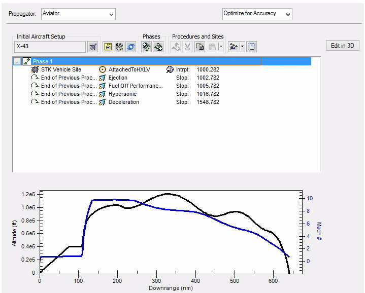
- Rename the aircraft X43_Notional.
The Profile Window should look similar to this:
3D View: Hypersonic flight window
View in 3D
Let's take a look at the flight in the 3D Graphics window.
- Set the Scenario Time Period to 1000.282 EpSec. This is the time the Hypersonic vehicle separates from the Pegasus.
- Zoom To the X43_Notional () in the 3D Graphics window.
- Animate (
 ) the scenario to watch the flight.
 - Pause (
 ) the animation when complete.
 - Save () the scenario.
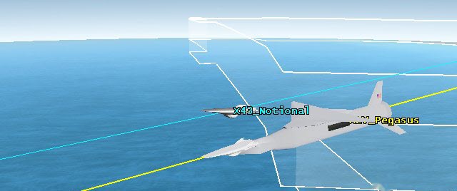
3D View: Hypersonic flight
Examine the Flight
The hypersonic flight was initially created with a low fidelity performance model. You can now compare it to the performance model based on the CFD data generated with ANSYS tools. This data is generated by running the X-43 in ANSYS Fluent at various stages throughout the flight envelope (varying velocity and angle of attack). From the CFD analysis, you were able to obtain the Coefficient of Lift (Cl) and Coefficient of Drag (Cd) values associated with each pair of AOA and velocity. With those values you were able to construct the performance profile for this vehicle.
Generate Downrange vs Altitude Graph
- Extend the Analysis menu.
- Open the Report & Graph Manager (
 ).
). - Set the Object Type to Aircraft.
- Select X43_Notional from the list of objects.
- Click the Create new graph style (
 ) button.
 - Set the Name to DownrangeVsAlt.
- Click Enter.
Define the Axis
- Set the Graph Type to XY.
- Expand the Flight Profile by Time directory.
- Set the X Axis to Downrange.
- Set the Y Axis to Altitude.
- Click .
Generate the graph
You can generate the data for more than one flight. To do this you can select both aircraft objects from the list.
- Multi-select the X43_Notional and HXRV_X43 from the list of aircraft.
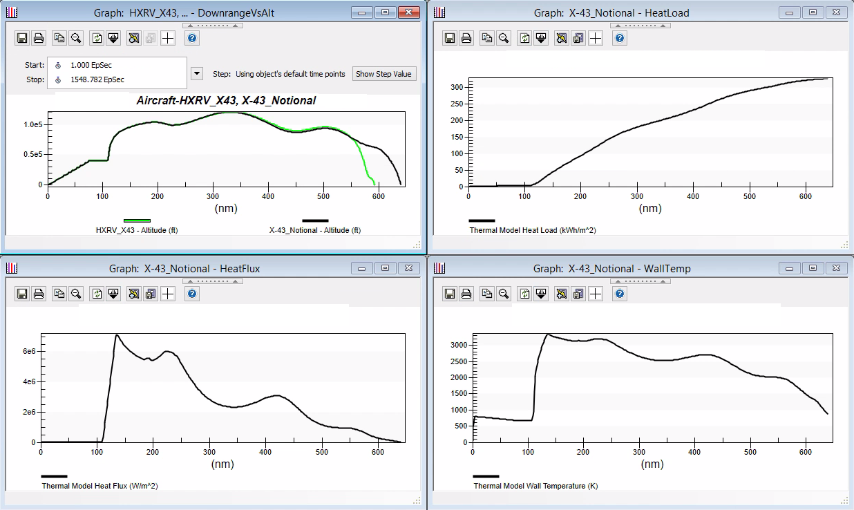
- Generate the DownrangeVsAlt graph.
- Examine the data and note the similarities and differences.
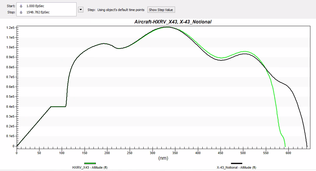
3D View: Hypersonic flight window
The X-43 flights (X43_Notional and HXRV_X43) have the same behavior, especially in the Hypersonic phase. The differences begin after the hypersonic phase. Both the CFD model (HXRV_x43) and the notional hypersonic model (X43_Notional) leverage the same aerodynamic specs of the hypersonic glider. The biggest difference is that the notional model uses internal physics to model the Cl and Cd of the aircraft. This is a general approximation of the flyout of the hypersonic vehicle. However, the CFD data provides a more accurate representation of the Cl and Cd of the aircraft.
Generate the Thermal Summary
STK v12.1 or newer provides thermal performance models to support the design and operations of hypersonic vehicles and related defensive systems. The X-43 thermal model from the initial setup can be reported on. If a hypersonic vehicle goes high and fast enough, users will see that the vehicle doesn’t get very warm on the boost, but gets very hot on the reentry. The more speed you add where the air is thin or nonexistent on the boost, the hotter it will get on reentry. For a depressed trajectory, the vehicle might get pretty hot during boost, it all depends on how much air there is, how fast the vehicle is moving, and the reference area of the leading edge.
It is important to model a system's thermal signature because it is of extreme interest to engineers and operators for both offensive and defensive systems. Lots of effort is being expended throughout the market on thermal environment effects for hypersonic vehicles. This feeds in to signature analysis. Structures and signatures and the areas those aspects drive are where a lot (if not most) of the money goes for both offensive and defensive systems. The ability to model this in STK, and move to the EOIR thermal models, makes it clear as to how detectable and, therefore, vulnerable a given trajectory is, and provides key measures for building these vehicles. Let's examine these parameters of our own hypersonic notional flight.
- Open the Report & Graph Manager ().
- Set the Object Type to Aircraft.
- Select X43_Notional from the list of objects.
- Click the Create new graph style () button.
- Set the Name to HeatFlux.
- Click Enter.
Define the Axis
- Set the Graph Type to XY.
- Expand the Flight Profile by Downrange data provider group.
- Set the X Axis to Downrange.
- Set the Y Axis to Thermal Model Heat Flux.
- Click OK .
Define the Head Load and Wall Temperate graphs
The Heat Load and the Wall Temperature are vital to know when modeling a hypersonic flight.
- Repeat the steps above to create graphs with the Thermal Model Heat Load and the Thermal Model Wall Temperature on the Y Axis.
- Rename the new graphs HeatLoad and WallTemp respectively.
Generate the graph
- Select the X-43_Notional from the list of aircraft.
- Generate the HeatFlux, HeatLoad, and the WallTemp graphs.
- Click OK on the Down Range Parameters pop up windows as the graphs are generating.
- Examine the data and note the increase in temperature as the Notional X-43 is ejected and reaches hypersonic speeds. When measuring the Wall Temperature, note that the temperature reaches ~3000 K. This will be relevant information when we examine a thermal infrared camera's ability to image this target.
Analyze the mission with EOIR
The flight is modeled and is being monitored by multiple systems around it. You can examine how a satellite tracks and views the hypersonic in flight. Using EOIR, you can build and analyze how well a system on-board a satellite would be able to image the hypersonic vehicle. Later you can examine how a UAV nearby would image the same target.
You can start by inserting a single satellite (not the full constellation from session 1) because for the scope of this study, you just want to understand how well the system on-board the satellite is able to image the X-43.
- Bring the Insert STK Objects tool () to the front.
- Insert a Satellite (
 ) using the Define Properties () method.
 - Set the following options:
- Click .
- Rename the satellite LEOSat.
| Option | Value |
|---|---|
| Semi-major Axis | 8112.14 km |
| Eccentricity | 0 |
| Inclination | 50 deg |
| Argument of Perigee | 0 deg |
| RAAN | 0 deg |
| True Anomaly | 60 deg |
This is just one satellite from the constellation that you will use to detect the X-43.
Insert a Sensor
- Using the Insert STK Objects tool, insert a Sensor (
 ) object using the Insert Default method.
 - When the Select Object window appears, select the LEOSat in the list and click .
- Rename the sensor Imager.
Define the sensor
Now that you have the sensor object in the scenario, let's define its properties.
- Open the Imager's () properties ().
- Browse to the Basic - Pointing page.
- Set the Pointing Type to Targeted.
- Move (
 ) HXRV_X43 to the Assigned Targets field.
 - Click on the properties.
- Save () the scenario.
This object has a predefined EOIR thermal model you can use.
EOIR Settings - Spatial
Set the EOIR spatial parameters for the sensor.
- Select the Basic - Definition page.
- Set the Type to EOIR.
- Select the Spatial tab.
- Set the following field-of-view options:
- Set the following number of pixels options:
- Click .
- Save () the scenario.
| Option | Value |
|---|---|
| Horizontal Half Angle | 0.002 deg |
| Vertical Half Angle | 0.002 deg |
| Option | Value |
|---|---|
| Horizontal | 1000 |
| Vertical | 1000 |
EOIR Settings - Spectral
The Spectral tab allows you to set the spectral band wavelengths. This study analyzes the Mid-wavelength infrared (3-5.5μm) otherwise known as the thermal infrared. This band allows you to narrow down the infrared signature of the hypersonic vehicle designed earlier in the lesson.
- Select the Spectral tab.
- Set the following Spectral Band Edge Wavelengths options:
- Click .
- Save () the scenario.
Enter the high number first to keep all values within the limits.
| Option | Value |
|---|---|
| High | 5.5 μm |
| Low | 3.0 μm |
EOIR Settings - Optical
On the optical tab you can set the Image Quality and the Optical Transmission. When you set the two optical inputs, the third is automatically calculated for you.
- Select the Optical tab.
- Set the following options:
- Leave the Optical Transmission and Diffraction Wavelength as the defaults.
- Click .
- Save () the scenario.
| Option | Value |
|---|---|
| Input | Focal Length and Entrance Pupil Diameter |
| Effective Focal Length | 415.00 cm |
| Entrance Pupil Diameter | 100.00 cm |
| Image Quality | Negligible Aberrations |
EOIR Settings - Radiometric
The radiometric tab allows you to define the radiant energy measurement properties. At a high level the sensitivity defines the noise floor of the sensor.
- Select the Radiometric tab.
- Ensure the Input to High Level.
- Leave all other parameters as the defaults.
- Click .
- Save () the scenario.
Examine the EOIR settings for the hypersonic vehicle
The sensor is now defined and you can see the thermal model of the hypersonic vehicle. The EOIR configurations have already been designed for the HXLV_X43. This was modeled in the starter scenario.
- Open HXRV_43's () properties ().
- Select the Basic - EOIR Shape tab.
- Ensure the Shape is set to CustomMesh.
- Ensure the Max Dimension is set to 30m.
- Confirm the Mesh File is set to x-43_eoir_v03.obj.
- Ensure the Material Specification is set to Geometric Groups.
- Examine the Material Elements and confirm the following values:
- Do not change any of the parameters.
- Click .
- Save () the scenario.
| Material Elements | Temperature |
|---|---|
| TopFront | 2931 K |
| TopBack | 3114 K |
| Stab_Vert_Outside | 3041 K |
| Stab_Vert_Inside | 3114 K |
| Stab_Horiz_Top | 3078 K |
| Stab_Horiz_Btm | 3078 K |
| Outlet | 3030 K |
| LeadingEdge | 3188 K |
| Intake | 2894 K |
| Inlet | 3151 K |
| Exhaust | 2600 K |
| BottomFront | 2790 K |
| BottomCenter | 3041 K |
| BottomBack | 3041 K |
These values were generated from ANSYS Fluent with the CFD results. The custom mesh you are designing is for the actual aircraft object itself. If you wanted, you could also model the plume coming from the vehicle to add another dimension on the synthetic scenes that would be generated.
Set up a target object
In the EOIR Target Configuration panel, users can select STK objects to use in the generated synthetic scene. You can add the HXLV_X43 to the list of objects. If the EOIR toolbar is not visible, then open the View - Toolbars menu and enable the EOIR option.
- Open the EOIR Target Configuration (
 ).
). - Move () the Aircraft/HXRV_X43 to the Selected Target field.
- Click .
- Save () the scenario.
Generate a synthetic scene
EOIR can create an image of what the system on the LEOSat would see. This sensor is tracking the hypersonic vehicle. You can jump to a moment in the scenario when the hypersonic vehicle is in view.
- Set the scenario time to 1200 EpSec. This is the time where the satellite is overhead of the test flight.
- Select the Imager ().
- Click the EOIRSyntheticScene (
 ) button. STK might take a few moments to generate the Synthetic Scene.
 - Use the scroll bars and the middle scroll of the mouse to resize the view.
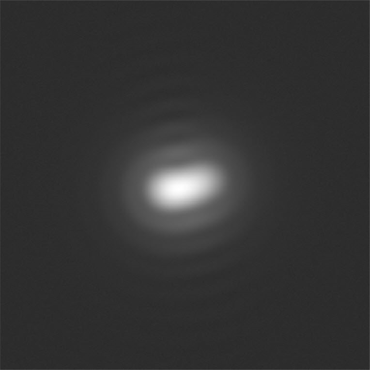
EOIR Synthetic Scene: Hypersonic flight
The HXRV_43 is approximately ~3500 km away at this point in time. This explains the low resolution of the synthetic scene.
Change the visual details
- Right-click in the Synthetic Scene window.
- Select the Details option.
- Set the Color Map to BGRY as the EOIR Scene Visual Details.
- Click .
- Close the Synthetic Scene.
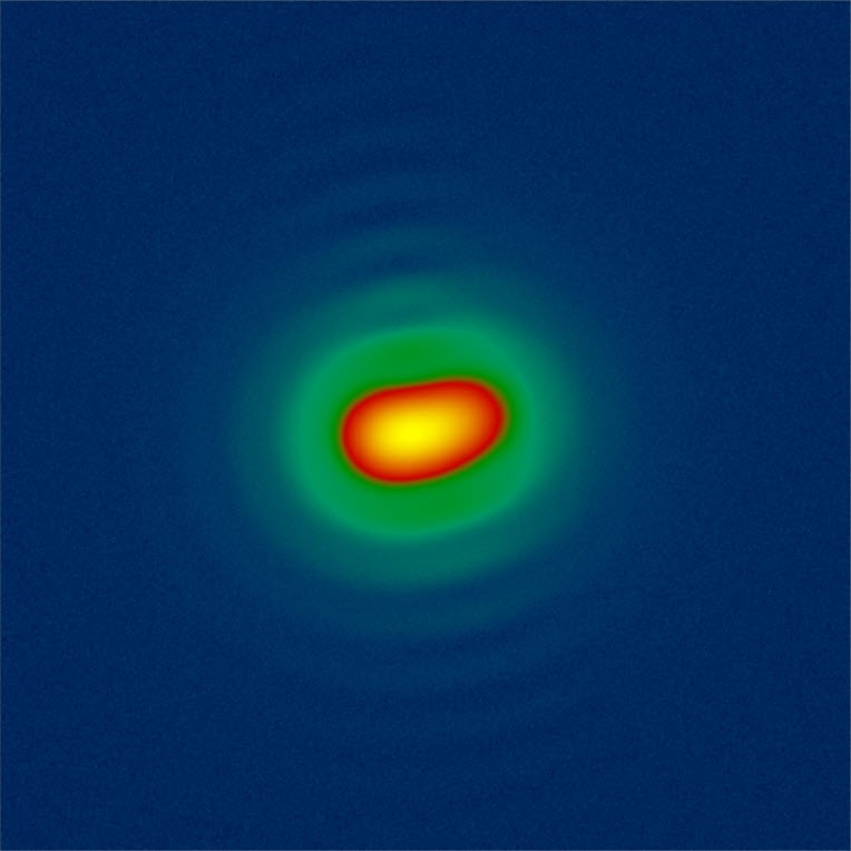
EOIR Synthetic Scene: Hypersonic flight BGRY
It is clearer to see the different thermal effects of the HXRV. However, this is still not as clear. Let's continue to examine the EOIR capabilities of STK; this time closer to Earth.
EOIR sensor on a UAV
EOIR sensors are flexible tools that be used in all domains. EOIR can create an image of what the system on a UAV flying near the HXRV can see. You can copy the sensor attached to the satellite to save on setup time.
- Copy the Imager () from LEOSat.
- Paste is on RQ-4B_Globalhawk ().
- Rename it UAV_Imager.
Modify the Field-of-View
The UAV is much closer to the HXRV. You can modify the field-of-view of the sensor because it does not need to be so small.
- Open UAV_Imager's () properties ().
- Browse to the Basic - Definition page.
- Ensure the Spatial tab is selected.
- Set the following options:
- Click .
- Save () the scenario.
| Option | Value |
|---|---|
| Horizontal Half Angle | 0.01 deg |
| Vertical Half Angle | 0.01 deg |
Generate a synthetic scene
- Set the scenario time to 1095 EpSec. This is the time that is the shortest distance between both objects.
- Select the UAV_Imager ().
- Click the EOIRSyntheticScene () button. STK might take a few moments to generate the Synthetic Scene.
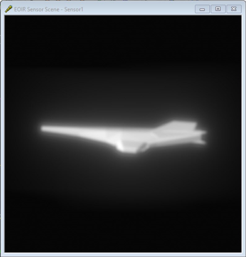
EOIR Synthetic Scene: Hypersonic flight
Notice the difference between the Imager on the satellite and the Imager on the UAV. The UAV is flying much closer to the HXRV and so it has a more defined synthetic scene. In this recreation of the hypersonic flight, you did not model the plume and just focused on the "what if" of a vehicle going this fast.
Examine the scene
Change the visual details
- Right-click in the Synthetic Scene window.
- Select the Details option.
- Set the Color Map to BGRY as the EOIR Scene Visual Details.
- Click .
- Select various points on the display to get additional data. Note the Temperature when clicking on various points of the X-43.
- Close the Synthetic Scene when done.
- Save () the scenario.
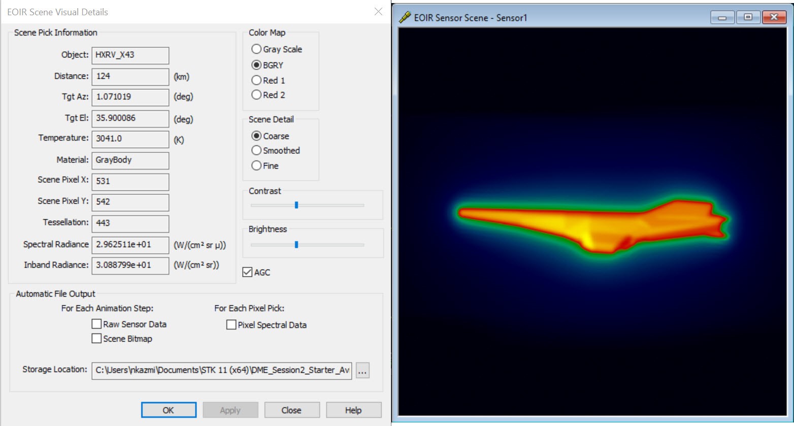
EOIR Synthetic Scene: Hypersonic flight BGRY with points selected
Analyze the Sensor System
Data providers allow users to pull relevant data from their mission. You can create a custom graph that measures the signal-to-noise throughout the flight.
- Open the Report & Graph Manager ().
- Set the Object Type to Sensor.
- Select the sensor attached to the RQ-4B_Globalhawk from the list of sensors.
- Click the Create new graph style () button.
- Rename the graph SNR_Hypersonic.
- Expand the EOIR Sensor To Target Metrics data provider.
- Double-click 'Signal to noise ratio' to add it to the Y Axis.
- Set the Step Size to 120 sec.
- Click .
EOIR can take a while to calculate, so it is a good idea to start with coarse settings and refine them later.
Generate the graph
- Double-click on SNR_Hypersonic to generate the graph.
- Select HXRV_X43 () as the target.
- Click . It may take a moment to generate the graph.
- Take a look at the results and notice how the system behavior changes over the time of the flight. Unlike the previous graphs of data we've looked at, the X-Axis is the time in the graph. We'll want to look at the behaviors of the HXRV_X43 at various times in the mission to understand the data.
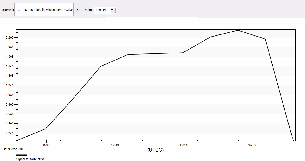
EOIR Synthetic Scene: EOIR sensor to Target Metrics
Modify the Time Step
The data from the graph is rough. Let's modify the time step to get additional information. This will take additional time to process (~45 min depending on your machine). Alternatively, you may use the image below as reference and jump to the times specified.
- Bring the graph to the front.
- Set the Step size to ten (10) seconds.
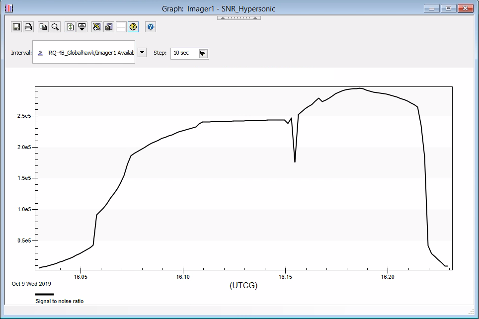
EOIR Synthetic Scene: EOIR sensor to Target Metrics with 10 second time step
From what we modeled of the launch, the first ~15 min (900 EpSec) are when the HXRV_X43 is attached to the HXLV_Pegasus. At ~925 EpSec there is a dip. The HXLV_Pegasus is raising to a higher altitude before the HXRV_X43 is deployed. Set the scenario time to 1000.00 EpSec and step forward in time to observe the deployment. It corresponds to the slight bump in the SNR before the peak. The peak at ~1100.00 EpSec corresponds to the moment the HXRV_X43 is the closest to the RQ-4B_Globalhawk, which is the platform for the thermal infrared sensor. Finally, recall that the HXRV_X43 descended into the ocean which can be followed in the remainder of the graph.
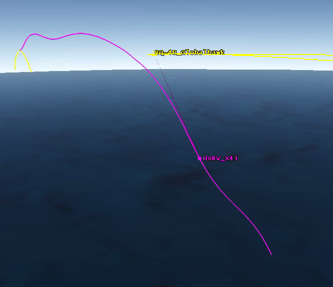
The HXRV_X43 Trajectory modeled using Aviator and imaged with EOIR
Closing
You have modeled the X-43 flight with a basic performance model and then compared that to a performance model derived from CFD using Aviator. With this tool, users can verify and validate their flights. Once the data is in STK, you can conduct post-flight analysis. With EOIR, users can model what their on-board systems see and how well they can detect an object traveling at Mach speeds.
DME Session 3
The next lesson in the DME series focuses on the test or mission planning phase of the lifecycle. Using the same models constructed through the design phase, you will evaluate relationships between assets like communications link availability and how that influences the overall mission timeline. You will bring the constellation from the first session and the flight from this session to understand how all components for the mission works together.