The Differential Corrector
(1)

where x is a vector of the independent variables - referred to as controls in Astrogator - and y is a vector of the dependent variables (results). The desired numerical values of the results are specified by yd. Evaluating the function f(x) involves propagating the segments in the target sequence with the specified x values, and computing the result variables y at the end state of the segments.
To find a solution for Equation 1, take a Taylor series expansion of f(x) to first order about the initial values of the control variables, x0
(2)
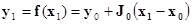
where the Jacobian, J, is the matrix of partial derivatives of the results for the controls
(3)
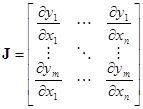
Here there are n control variables and m result variables. The Jacobian is also known as the sensitivity matrix because it shows how sensitive the result variables are to changes in the control variables.
To solve for the control values that will yield the desired values of the results, rearrange Equation 2 as(4)
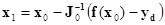
where J-1 indicates the pseudo-inverse when J is not square (n≠m). But, because Equation 2 is a truncated Taylor series, the expression in Equation 4 only gives an approximate solution. If the error, f(x1) – yd, is above tolerance then repeat the process. This algorithm can be expressed as
(5)
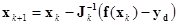
where k is the iteration number. The process repeats until the error is below tolerance for each result variable. Since J-1 appears in Equation 5, the Jacobian matrix must be invertible for the differential corrector to perform correctly, so there must not be any degeneracy in the matrix. In Astrogator, the inverse is computed with a singular value decomposition (SVD) algorithm.
The algorithm requires computing the partial derivatives that comprise the Jacobian. The derivatives are approximated by numerical differentiation (forward or central difference), where f(x) is evaluated with the control variables perturbed by small amounts δx. With forward differencing, the default option in Astrogator, the ith column of J is given by
(6)
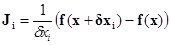
where the scalar δxiis the perturbation of the ith control variable and the vector δxi is
(7)
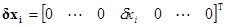
In Astrogator, you can enter the value of the perturbation δxi in the Perturbation field for the appropriate variable in the targeter, or you can let Astrogator use a default value.
Computing J numerically requires n evaluations of f(x). After using Equation 5 to find the values to use for the control variables, run a final evaluation to see if the result variables are within tolerance of their desired values. If they are not, run another iteration. Thus, for a problem with n independent variables, each iteration requires n+1 evaluations. Because an evaluation is also required before the first iteration to compute the initial values of the dependent variables, a solution in k iterations requires (n+1)k + 1 evaluations. The approach described here, where numerical derivatives are used to compute J, is a classic Newton-Raphson implementation of the differential corrector.
Instead of numerically computing the partials that comprise J on every iteration, an approximation to J can be used that is based on the change to the result variables on each iteration. This technique is a generalized secant method, also called Broyden’s method. The approximation, , is given by
(8)
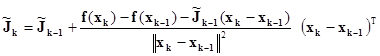
When the secant method is used, the initial value of the Jacobian, , is found in the first iteration using numerical derivatives as it is in Newton-Raphson. Because of the initial evaluation, with n independent variables this first iteration requires n+2 evaluations. On later iterations Equation 8 is used, only requiring a single evaluation of f(x). Thus, a solution in k iterations of a problem with n independent variables requires k + n + 1 evaluations. The number of evaluations per iteration with the secant method is less than it is with the Newton-Raphson method. But, the secant method may require more iterations to converge to a solution than Newton-Raphson because Equation 8 is just an estimate of the actual Jacobian values computed in Equation 6.
A special case arises with the secant method in targeting problems with multiple control variables but only a single result variable. In this case the Jacobian is a column vector. Because the step taken in the control variables is in the same direction as that column vector, updates to J through Equation 8 will also be in the same direction. If Equation 8 was used on every iteration and the solution was not along that line, the method would never converge. So, when there are multiple control variables but only one result variable, Astrogator re-computes the Jacobian with Equation 6 whenever the solution starts to diverge. Divergence is detected whenever the result is further from its desired value than it was on the previous iteration.
More information about how the Newton-Raphson and secant methods are implemented in Astrogator, and comparisons between using the methods to solve trajectory problems can be found in the paper, Comparisons between Newton-Raphson and Broyden's methods for trajectory design problems, by Matthew M. Berry.