STK Premium (Space) or STK Enterprise
You can obtain the necessary licenses for this tutorial by contacting AGI Support at support@agi.com or 1-800-924-7244.
The results of the tutorial may vary depending on the user settings and data enabled (online operations, terrain server, dynamic Earth data, etc.). It is acceptable to have different results.
Capabilities covered
This lesson covers the following capabilities of the Ansys Systems Tool Kit® (STK®) digital mission engineering software:
- STK Pro
- STK SatPro
- Conjunction Analysis
Problem statement
Satellite analysts need a quick way to simulate and determine the probability of collision between their satellite and any other satellites in orbit. Two satellites are in close proximity of each other. You need to determine the distance between the satellites at the time of closest approach, based on a fixed threat volume and object location and determine the probability of collision. You also need to determine if the conjunction's relative motion appears linear or nonlinear. Covariance data is available and required for the analysis.
Solution
Use the STK software's Conjunction Analysis capability to carry out a close-approach analysis for the satellites. You'll also perform a close approach analysis between the primary object (your satellite) and the secondary object (the satellite presenting a risk of collision), with reference to a threshold. The threshold is the minimum acceptable distance between the ellipsoidal threat volumes of the objects and the range between the objects. Then, you'll apply covariance data to the analysis. Using the Nonlinear Probability Tool, you'll determine if the conjunction is linear or nonlinear.
What you will learn
Upon completion of this tutorial, you will understand how to:
- Use the High-Precision Orbit Propagator (HPOP)
- Use the Conjunction Analysis capability
- Use the Advanced CAT tool
- Use the Nonlinear Probability Tool
- Create custom reports using the Report & Graph Manager
Creating a new scenario
First, you must create a new STK scenario, and then build from there.
- Launch the STK application (
 ).
). - Click
 Create a Scenario when the Welcome to STK dialog box opens.
 - Enter the following in the STK: New Scenario Wizard:
- Click when you finish.
- Click Save (
 ) when the scenario loads. The STK application creates a folder with the same name as your scenario for you.
 - Verify the scenario name and location in the Save As dialog box.
- Click .
| Option | Value |
|---|---|
| Name | Conjunction_Analysis |
| Start | 1 Jun 2019 16:00:00.000 UTCG |
| Stop | 4 Jun 2019 16:00:00.000 UTCG |
Save (![]() ) often during this scenario!
) often during this scenario!
Removing unneeded windows
The Timeline View and the 2D Graphics window are not required for this scenario, so you can remove them from your workspace.
- Close (
 ) the Timeline View.
 - Close () the 2D Graphics window.
Creating the primary satellite
Two satellites are required in the analysis. One satellite, Primary, is prebuilt and is saved as an ephemeris file. An ephemeris file is an ASCII text file formatted for compatibility with the STK software that ends in a *.e extension. You can generate an ephemeris file with the High-precision Orbit Propagator (HPOP) using a frame defined by a Conjunction Data Message (CDM). The CDM specification allows many possible frames, but having all the data in ephemeris files where the frame is specified in the metadata allows for the appropriate comparisons. An ephemeris file may also contain covariance data.
If you have your ephemerides converted to ephemeris files (regardless of the frame), the STK application will handle all the conversions internally for whatever analysis it needs to perform. The bottom line is that the STK application needs *.e files, manually entered satellite properties, or
Inserting a new Satellite object
Primary is your primary satellite of interest. The satellite was built using the HPOP propagator and was saved as an ephemeris file.
- Bring the Insert STK Objects tool (
 ) to the front.
 - Select Satellite (
 ) in the Select An Object To Be Inserted list.
 - Select Insert Default () in the Select A Method list.
- Click .
- Right-click on Satellite1 () in the Object Browser.
- Select Rename in the shortcut menu.
- Rename Satellite1 () Primary.
Using the StkExternal propagator
The SatPro capability extends the STK software into the realm of high-fidelity satellite systems modeling and analysis. The propagators included in SatPro can incorporate numerical integration and differential equations of motion, compute ephemeris for months and years, and integrate specialized propagation methods. The
- Right-click on Primary () in the Object Browser.
- Select Properties (
 ) in the shortcut menu.
 - Select the Basic - Orbit page.
- Open the Propagator drop-down list.
- Select StkExternal.
- Click the Filename ellipsis (
 ).
). - Browse to the location of the ephemeris file in the STK software installation directory, typically <Install Dir>\Data\Resources\stktraining\text when the Select an Ephemeris File dialog box opens.
- Select Primary.e.
- Click .
- Click to accept your selections, to propagate Primary () and to close the Properties Browser.
Creating the secondary satellite using the High-precision Orbit Propagator (HPOP)
The High-precision Orbit Propagator (HPOP) included with the SatPro capability uses numerical integration of the differential equations of motions to generate ephemerides. When you use the HPOP propagator, you can choose from several numerical integration techniques and formulations of the equations of motion. You can also include force modeling effects, such as a full gravitational field model (based upon spherical harmonics), third-body gravity, atmospheric drag, and solar radiation pressure.
HPOP can handle the following orbit types:
- circular
- elliptical
- parabolic
- hyperbolic
The orbits can be propagated around any central body and at distance ranges from the lower atmosphere of the Earth, to the Moon, and beyond.
You will build the secondary satellite using orbital parameters obtained from an external source, such as a CDM. There are various ways to enter data for Satellite object. For this scenario, you will manually enter orbit coordinates after choosing HPOP as the Satellite object's propagator and then transfer in covariance data using a Connect command. The Connect command is entered using the API Demo Utility, but the covariance data could be sent from outside of STK using other means (for example, Excel, MATLAB, a script, etc.).
This section contains important information that users of the STK software should read. If you don't want to manually insert the secondary satellite, however, skip this section and start at the
Creating a new Satellite object
Insert a new satellite using the Insert Default method.
- Bring the Insert STK Objects tool () to the front.
- Insert a Satellite () object using the Insert Default () method.
- Rename Satellite2 () Secondary.
Selecting the High-precision Orbit Propagator
Select HPOP as Secondary's propagator and manually enter the orbital parameters.
- Open Secondary's () Properties ().
- Select the Basic - Orbit page.
- Set the Propagator to HPOP.
- Set the following orbital parameters:
- Click to accept your changes and to keep the Properties Browser open.
| Option | Value |
|---|---|
| Step Size | 6 sec |
| Coord Type | Cartesian |
| X | -7669168.8042875 m |
| Y | -7859650.1453306 m |
| Z | -23040324.781931 m |
| X Velocity | 2232.2151237860 m/sec |
| Y Velocity | -3239.6197689674 m/sec |
| Z Velocity | 358.11070444968 m/sec |
When entering the data, it is a good idea to copy and paste the Cartesian Coordinates from this tutorial directly into the STK application.
Using force models
You can use force models to define a precise representation of a satellite's force environment for use in HPOP analysis. The focus of this tutorial is the Advanced CAT tool, but you'll make some changes to the force models to align them with the models used to generate ephemeris for the primary satellite.
- Click .
- Ensure the Gravity tab is selected when the Force Model Properties - Secondary dialog box opens.
The gravity tab of the HPOP Force Model Properties window enables you to configure a central body gravity model, solid and ocean tide effects, and third body gravity effects.
Selecting the gravity file
The gravity field of a central body is an extremely important constituent of the total force model on a body. Gravity field information is contained within a formatted ASCII text file called a
- Click the Gravity File ellipsis () in the Central Body Gravity panel.
- Select WGS84_EGM96.grv in the Select a Gravity Field dialog box.
- Click .
Updating the Central Body Gravity force model parameters
Update the maximum degrees and order of the geopotential coefficients to be included for the Central Body gravity computations. The range of values is enforced by the central gravity model (*.grv) you set.
- Enter the following Central Body Gravity parameters:
- Clear the Truncate to Gravity Field Size check box in the Solid Tides panel.
- Clear the Use check boxes for Sun and Moon in the
| Option | Value |
|---|---|
| Maximum Degree | 0 |
| Maximum Order | 0 |
Besides earth gravity, you can model the effects of gravity from a third body on your satellite's orbit behavior. The Third Body Gravity table is ordered to reflect the maximum possible third-body force produced by each central body, when that body is located at its closest to the Earth. For this scenario, however, you want to exclude the gravitation pull from the Sun and Moon from the force computations.
Discounting drag and solar radiation pressure
For this scenario, you do not want to model the effects of drag or solar radiation pressure (SRP) in the HPOP trajectory calculation.
- Select the Drag tab.
- Clear the Use Drag check box.
- Select the SRP tab.
- Clear the Use SRP check box.
- Click to accept your changes and to close the Force Model Properties - Secondary dialog box.
- Click to accept your changes and to keep the Properties Browser open.
Propagating covariance
HPOP is capable of
State error covariance growth is usually dominated by the initial position and velocity covariance which is typically generated by orbit determination software. Any errors between the estimated state and the actual state tend to grow over time especially in the along-velocity direction. This is a direct effect of the dominant two-body force since the period of the orbital motion is on its initial state. Eccentric orbits also show a oscillation in uncertainty superposing the growth trend which has a larger amplitude for larger eccentricity. Uncertainty increases near perigee where the speed of the vehicle is largest in its orbital cycle. Uncertainty will actually decrease near apogee where the speed is the smallest.
A second contributor to state error covariance growth is force model mismodeling. The force model environment modeled by the software, chosen by you to best represent the force environment, does not precisely model the actual forces experienced by the vehicle. In orbit determination software that uses Kalman or related filters, force model mismodeling contributes to covariance growth through process noise models that aim to characterize the uncertainty of the modeling itself. Because HPOP does not have all the data needed to do this sophisticated analysis, it uses a simpler scheme to account for some force model mismodeling called "consider analysis."
A consider analysis adds contributions of force model mismodeling to the state error covariance propagation by treating constant parameters in the force model as being instead uncertain themselves. The uncertainty in the parameter value leads to uncertainty in the force evaluation which then contributes to the state error covariance.
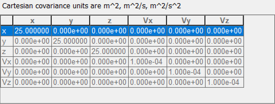
In the absence of an external ephemeris file, the HPOP propagator is used to propagate satellite position, velocity and associated covariances. The Covariance page enables you to enter your initial state error covariance matrix. Because the matrix is symmetric, you only need to enter the lower triangle.
Cartesian covariance units are m2, m2/s, m2/s2.
- Click .
- Click to close the HPOP Covariance - Secondary dialog box.
- Click to accept your changes and to close the Properties Browser.
Default Cartesian Covariance Units
You could manually enter the Cartesian covariance units from the CDM. To save time, however, you'll use a pre-constructed Connect command to enter the data.
Using the HPOP Covariance Connect command
The HPOP Covariance command enables you to enter an initial state error covariance matrix using Connect. In this instance, set the position velocity (PosVel) parameters. To enter the HPOP Covariance Connect command, use the API Demo Utility.
- Click New Web Browser Window (
 ) in the STK toolbar.
 - Click Browse (
 ) in the Web Browser - AGI - Resources web browser toolbar.
 - Select the Example HTML Utilities folder in the Navigation pane when the Open dialog box opens.
- Select the STK Automation folder .
- Click .
- Select the API Demo folder.
- Click .
- Select API Demo Utility.
- Click .
Sending the HPOP Connect command to Secondary
Copy and paste the completed HPOP Connect command into the API Demo Utility Code Sandbox.
- Copy and paste the 21 values representing the lower triangle of the 6×6 position velocity submatrix in the Code Sandbox of the Web Browser - API Demo Utility.
- Click .
- Close () the Web Browser - API Demo Utility.
hpop */Satellite/Secondary Covariance PosVel 0.55964154920517E-01 -0.23168820659027E-01 0.73624971281146E-01 0.25611038576040E-02 -0.37169368664612E-02 0.40410873798337E-01 0 0 0 0.10000000000000E-07 0 0 0 0.70962140501337E-24 0.10000000000000E-07 0 0 0 0.35340968553901E-25 -0.24799262505252E-24 0.10000000000000E-07
You can also enter the parameters manually if needed.
Syntax:
PosVel <xx> <yx> <yy> <zx> <zy> <zz> <Vxx> <Vxy> <Vxz> <VxVx> <Vyx> <Vyy> <Vyz> <VyVx> <VyVy> <Vzx> <Vzy> <Vzz> <VzVx> <VzVy> <VzVz>
Viewing the state error covariance matrix
You want to ensure that the state error covariance matrix was updated using the Connect command.
- Open Secondary's () Properties ().
- Selct the Basic - Orbit page.
- Click .
- Select the Compute Covariance check box in the HPOP Covariance - Secondary dialog box to include covariance in Secondary's propagation.
- Enter the following in the Gravity panel:
- Check the Cartesian covariance units.
- Click to close the HPOP Covariance - Secondary dialog box.
- Click to accept your changes and to keep the Properties Browser open.
- Skip to the Controlling the display of satellite orbits in the 3D Graphics window section.
| Option | Value |
|---|---|
| Maximum Degree | 0 |
| Maximum Order | 0 |
You're matching the force model gravity values set earlier in the scenario.
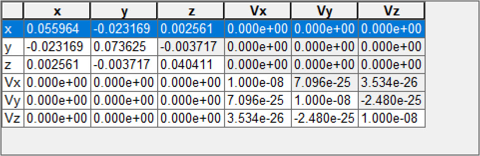
Inserted Cartesian Covariance Units
The Cartesian covariance units should have been populated with the values sent from the Connect command.
Creating the secondary satellite using an ephemeris file
Use this section if you're using the prebuilt secondary satellite.
- Insert a Satellite () object using the From External Ephemeris File (*.e) (
 ) method.
 - Browse to the location of the ephemeris file, typically <Install Dir>\Data\Resources\stktraining\text in the Select an Ephemeris File dialog box.
- Select Secondary.e.
- Click .
- Rename Satellite2 () to Secondary.
- Open Secondary's () Properties ().
- Select the Basic - Orbit page.
- Click .
- Click to accept your changes and to keep the Properties Browser open.
Controlling the display of satellite orbits in the 3D Graphics window
The Lead Type defines the display of the leading portion of a vehicle's track. Update Secondary's
- Select the 3D Graphics - Pass page.
- Open the Lead Type drop-down list in the Orbit Track panel.
- Select All.
- Click to accept your changes and to keep the Properties Browser open.
Changing the orbit system view
Show Secondary's orbit in an object-centered Vehicle Velocity Local Horizontal (VVLH) reference frame with the Z axis opposite the position vector and the X axis toward the inertial velocity vector.
- Select the 3D Graphics - Orbit System page.
- Clear the Inertial by Window - Show check box.
- Click .
- Select Primary () in the in the VVLH System Object panel of the Select Object VVLH System dialog box.
- Click to close the Select Object VVLH System dialog box.
- Click to accept your changes and to close the Properties Browser.
Viewing both satellites
The motion of the secondary satellite is relative to the primary satellite; that is why it is being shown in the VVLH frame of the primary satellite. Each loop corresponds to one orbit revolution.
- Bring the 3D Graphics window to the front.
- Right-click on Primary () in the Object Browser.
- Select Zoom To.
- Use your mouse to refine your view until you can see both satellites.
- Click Increase Time Step (
 ) in the Animation tool bar and set the Time Step to 300 sec.
 - Click Start (
 ) to animate the scenario.
 - Click Reset (
 ) when finished.
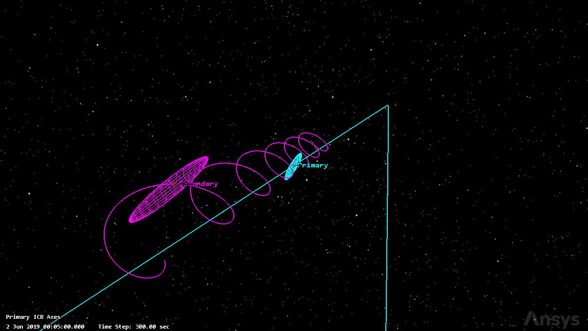
Primary and Secondary Satellites
Notice how that
Using the Advanced CAT tool for conjunction analysis
You will complete a linear and a nonlinear analysis. Start with a linear analysis using the Conjunction Analysis capability. The Conjunction Analysis capability's
Customizing the Insert STK Objects tool
The AdvCAT object provides a convenient way to launch the Advanced CAT tool. However, to use it, you must first add the AdvCAT object to the Insert STK Objects tool.
- Bring the Insert STK Objects tool () to the front.
- Click .
- Select the AdvCAT check box in the New Object list when the Preferences dialog box opens.
- Click to close the Preferences dialog box.
- Insert an AdvCAT (
 ) object using the Insert Default () method.
Setting Advanced CAT properties
The
- To use the Advanced CAT tool, click the Advanced CAT icon in the Object Catalog.
- Open AdvCAT1's () Properties ().
- Select Satellite/Primary in the Available list of the Primary List panel.
- Move (
 ) Satellite/Primary to the Chosen list.
 - Select Satellite/Secondary in the Available list of the Secondary List panel.
- Move () Satellite/Secondary to the Chosen list.
- Click to accept your selections and to keep the Properties Browser open.
Note the default threshold of 10 km. This is the threat volume and you can change it if required. Advanced CAT assigns to each primary and secondary satellite a threat volume, comprising an ellipsoidal shape enclosing the object. This shape possibly represents the degree of uncertainty regarding an object's position at any given time. When the range between ellipsoids falls below the user-selected threshold, STK issues a warning . A collision event occurs whenever the range between the two threat volumes becomes zero or negative.
As you move down the page, primary objects are the satellites of interest to you, such as those that you own or wish to use. Secondary objects are those that present a potential risk of collision with, or unacceptably close approach to, your primary objects.
Setting fixed definition ellipsoid values
You can select the approach for the STK software to take to determine the dimensions of the threat volume. Begin by using a Fixed definition type, which is the default class. The Fixed definition specifies the dimensions of the threat volume ellipsoid on the basis of values you enter.
- To edit the Tangential, Cross Track, and Normal dimensions of an object's threat volume (with Fixed selected as the Class), enter the desired values directly in the grid. Set the following values for both the Primary and Secondary satellites:
- The X axis is in the tangential direction, i.e., parallel to the object's velocity vector.
- The Y axis is in the cross-track direction, i.e., parallel to the orbit normal vector, or the cross product of the radius and velocity vectors.
- The Z axis is in the normal direction, i.e., parallel to the cross product of the X and Y axes.
- The X and Z axes are in, and the Y axis is perpendicular to, the orbit plane.
- HardBodyRadius displays the Hard Body Radius value for each object in the Primary and Secondary lists.
- Click to accept your selections and to keep the Properties Browser open.
| Option | Value |
|---|---|
| Tangential | 10 km |
| CrossTrack | 5 km |
| Normal | 5 km |
| HardBodyRadius | 0.002 km |
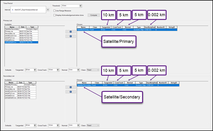
Proper Settings
Reviewing advanced options
The
- Select the Basic - Advanced page.
- Note the various fields and settings.
- You will use the default settings on this page.
On the Basic - Main page, the Threshold is set to 10 km. On the Basic - Advanced page, default Pre-Filters are set to Apogee/Perigee 30 km and Time to 30 km. If you make any changes to the Pre-Filters, make sure they are equal to or greater than the threshold.
For advanced technical information, refer to Salvatore Alfano and David Finkleman's white paper, "Operating Characteristic Approach To Effective Satellite Conjunction Filtering".
Computing a linear conjunction analysis
With your parameters set, launch the close approach computation process.
- Select the Basic - Main page.
- Click .
Creating a custom report
The AdvCAT object provides numerous data provider elements for Events by Min Range. Understanding these choices enables you to determine which elements are needed in your analysis.
Creating a custom report style
Duplicate the existing Close Approach By Min Range report style so you can customize it further.
- Right-click on AdvCAT1 () in the Object Browser.
- Select Report & Graph Manager... (
 ) in the shortcut menu.
 - Select the Close Approach By Min Range (
 ) report in the Installed Styles (
 ) folder in the Styles panel of the Report & Graph Manager.
 - Click Duplicate style (
 ) in the Styles panel toolbar.
 - Select the Content page.
Selecting data providers and elements
You will add six additional data provider elements to your custom report.
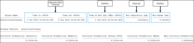
- Time at Min Sep (TMS): The time of the minimum separation between the primary and secondary threat volumes.
- Collision Probability (Analytic): The probability of collision computed using an analytic method based upon Ken Chan's paper. Chan (Aerospace) transforms the two-dimensional Gaussian probability density function (pdf) to a one-dimensional Rician pdf and uses the concept of equivalent areas.
- Collision Probability (Numeric): The probability of collision computed using a numeric method based upon Sal Alfano's paper. Collision Probability (Numeric) will return -1.0 as an error indicator when encounter plane's sigma X or sigma Z value is too small (less than 0.1 mm).
- Collision Probability (Patera 2005): The probability of collision is computed using an analytic method based upon Russell Patera's paper that appeared in the Journal of Guidance, Control and Dynamics, vol. 28 (6), 2005.
- Collision Probability (Maha): The probability of collision computed based on the Mahalanobis distance method. The Mahalanobis distance is the distance between two points in multivariate space. The Mahalanobis distance is a measure of the distance between a point P and a distribution D, introduced by P. C. Mahalanobis in 1936.
- Max Collision Probability: The maximum probability of collision, as defined by Sal Alfano's paper.
- Select the Events by Min Range-Time Out in the Report Contents list.
- Select the Time at Min Sep (TMS) (
 ) data provider element in the Data Providers list.
 - Click Insert ().
- Select Events by Min Range-Min Range in the Report Contents list.
- Click .
- Click .
- Insert () the following data provier elements to Section 6 Line 1.
- Collision Probability (Analytic) ()
- Collision Probability (Numeric) ()
- Collision Probability (Patera 2005) ()
- Collision Probability (Maha) ()
- Max Collision Probability ()
- Click to accept your selections and to close the Properties Browser.
This takes you to the location of the element in the data providers list.
Renaming your custom report
Give your report a new name to better differentiate it from the default report.
- Right-click on Close Approach By Min Range (
 ) in the My Styles () folder.
 - Select Rename in the shortcut menu.
- Rename Close Approach By Min Range () Custom Close Approach By Min Range.
- Click .
Understanding the data
As you scroll down through the report, focus on the last two lines. Your report's values may be different from the image (different data entered, etc.). The purpose of the image is to explain the data provider elements.
Linear Data
- Leave the Report open.
- Close the Report & Graph Manager.
Factoring covariance into the analysis
Now you will take covariance into consideration. Use the positional covariance associated with the object to determine the size and orientation of the threat volume ellipsoid.
- Return to AdvCAT1's () properties.
- Click on Fixed in the Chosen - Class cell in the Primary List panel.
- Open the drop-down list.
- Select Covariance.
- Set Satellite/Secondary's class to Covariance.
- Click to accept your changes and to keep the Properties Browser open.
- Click .
- Click to accept your changes and to close the Properties Browser.
Refreshing your custom report
Refresh your custom report to view the changes.
- Bring the Custom Close Approach By Min Range report to the front.
- Click Refresh (F5) (
 ) in the report toolbar.
 - Close the report when finished.
Note that the collision probability changes. It's increased substantially. However, the minimum range is still the same.
Using the Nonlinear Probability Tool
The previously mentioned methods (Chan, Alfano, Patera, and Maha) all assume linear relative motion; that is to say, the secondary satellite moves past the primary satellite in a straight line. Under certain circumstances (GEO orbits, rendezvous, formation flying, etc.) this assumption is violated, as seen in the 3D Graphics window (Primary and Secondary orbits). However, the Conjunction Analysis capability provides you with a tool to determine when the linear assumption is not valid.
The Nonlinear Probability Tool can be used to compute conjunction probability for nonlinear relative motion. The tool enables you to test for linear relative motion and provides two methods for computing conjunction probability: adjoining parallelepipeds (bundles) and adjoining tubes (cylinders). If the test shows you have a nonlinear conjunction, you should use one of these methods to obtain a proper probability of collision.
Addressing nonlinear motion using cylinders
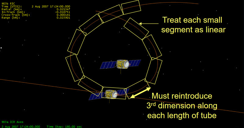
Analyzing Non Linear Motion Using Cylinders
Computing probability of collision using cylinders is done by breaking the collision tube into smaller sections, computing the probability associated with each section, and then summing.
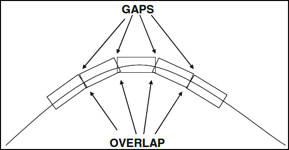
Overlapping Cylinders
Nonlinear motion causes gaps and overlaps where the tube sections meet. If the relative motion track bends towards the covariance ellipsoid center, then the overlapping sections will occur in regions of greater probability density with the gaps occurring in regions of lesser probability density. Although the gap and overlapping volumes are almost equal, their probability densities are not. The resulting summation causes an overinflation of the probability. If the relative motion track bends away from the covariance ellipsoid center, then the probability for cylindrical tubes will be underestimated because the gap is in a region of higher probability density. The amount of error will vary based on the degree of bending / overlap relative to probability density.
Addressing nonlinear motion using bundles
The gaps and overlaps created by adjoining right-circular cylinders can be reduced by sectioning the cylinder into component pieces. The gaps and overlaps of all the sections will be considerably smaller than the unsectioned cylinder. If there is sufficient movement in the probability density space, the aforementioned discs can be linked to form a bent collision tube. The right cylinders described in the previous section are replaced by bundles of abutting parallelepipeds. Each parallelepiped end is adjusted such that the bundle forms a compound miter where neighboring tubes meet, thereby reducing the gaps and overlaps of the previous method. The implicit assumption is that the one-dimensional probability along the central axis of each parallelepiped adequately represents that dimension’s probability for any point on the face of the parallelepiped.
Opening the Nonlinear Probability Tool
Open the Nonlinear Probability ool from the Object Browser.
- Select AdvCAT1 () in the Object Browser.
- Select AdvCAT in the shortcut menu item.
- Select Nonlinear Probability... in the AdvCAT submenu.
Understanding the Nonlinear Probability Tool interface
At the top of the Nonlinear Probability Tool are Primary Object, Secondary Object, and Time of Closest Approach lists. If you were working with more than one satellite, the lists display them. If all three fields are blank, click . This could be the case if you shut down the STK application and restarted your scenario at a later time.
- Review the End Sigma field.
- 1 sigma ≥ 19.87%
- 2 sigma ≥ 73.85%
- 3 sigma ≥ 97.07%
- 4 sigma ≥ 99.89%
- 5 sigma ≥ 99.998%
- 6 sigma ≥ 99.99999%
- Review the Fractional Limit of Probability field.
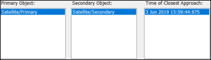
Objects and TCA
The End Sigma field holds a default value of 4.000. This enables you to set your probability density. 3D sigmas contain the following probability densities:
You can see that you do not gain much beyond 4 sigma. This is operator defined based operational requirements. Keep the default value.
The Fractional Limit of Probability is the acceptable difference between linear and nonlinear computations. This is operator defined based on operational requirements. Keep the default.
Testing for nonlinearity
Perform the linearity test and review the results to see if a nonlinear computation is warranted.
- Click .
- Read the information in the Warning dialog box.
- Click to close the Warning dialog box.
- Review the results in the Dilution, Maximum Prob, and Linear Prob fields.
- Dilution: the dilution distance should be compared to the predicted miss distance. If miss distance is less than dilution distance, then you are in the dilution region. This is an indicator that you should try to get better data, perhaps an update and / or prioritized tracking.
- Maximum Prob: the maximum probability computation scales and reorients the original covariance at time-of-closest-approach (TCA) to produce a maximum. This is a "worst case" number if you do not have confidence in your covariance or if covariance is not provided (such as with TLEs).
- Linear Prob: the linear probability is the estimated actual probability assuming linear relative motion at TCA. It can be used to compare / contrast with the nonlinear results, which you'll see later.
- Review the results in the TCA Rel Val and Approx Min Rel Val fields.
- TCA Rel Vel: this is the velocity of Secondary relative to Primary.
- Approx Min Rel Vel: this is the relative speed that must be matched or exceeded for the conjunction to be considered linear based on the Fractional Limit of Probability threshold.
The warning notes your conjunction appears to be nonlinear.

Dilution, Maximum and Linear Probabilities
Note that a red X (![]() ) has appeared next to the Approx Min Rel Vel field. This confirms your conjunction is nonlinear.
) has appeared next to the Approx Min Rel Vel field. This confirms your conjunction is nonlinear.
Computing collision probability using cylinders
You determined your conjunction is nonlinear. Now, use the cylinders method to compute a proper probability of collision. For the purposes of this tutorial, a probability of ≥ 1e-4 meets some form of reporting criteria. Based on the reporting criteria, a probability of collision greater than or equal to 0.0001 requires action.
- Review the following fields:
- Max Time Step: this sets the sectional time step upper limit. Leave the default.
- Max Angular Bend: this limits the angular difference between abutting cylinders. A higher number could create larger cylinder gaps. Leave the default.
- Max Sigma Step: this limits individual cylinder length based on the traversed Mahalanobis distance. Leave the default.
- Enter 0 sec in the Integration Duration field.
- Click .
- Take a look at the results.
The Integration Duration field defines the span of time that will be evaluated. By default, this span is defined as one half of the orbital period, since an integration duration of one quarter of the orbital period forward and backward from TCA is recommended. Setting this value to 0 sec achieves this goal for you.
The probability of collision is rather high. Remember, cylinders contain gaps and overlaps which can produce an over inflation of the probability.
Computing collision probability using bundles
Using cylinders, the probability of collision exceeded the criteria for reporting a possibility of collision. Now compute the conjunction probability using the bundles method.
- Leave the Resolution set at 0.0001 km.
- Click .
- Compare the Cylinders and Bundles probability value to the Linear probability value.
- Click to close the Nonlinear Probability Tool when finished.
You must specify how many parallelepipeds are needed to adequately represent the combined object space; the Resolution field defines this granularity for the two-dimensional probability computation by determining grid size.
The probability of collision is higher than when using cylinders, which is expected. However, the value using the cylinders method is well with range of taking some form of action. You could have used those numbers alone.
Saving your work
Clean up your workspace and save your work.
- Close any open reports, properties and tools.
- Save () your work.
Summary
You began by loading a prebuilt ephemeris file for the primary satellite and manually loading properties for the secondary satellite. You could load your values into a Satellite object's properties from outside of the STK application using a script or the STK software's Integration capability and an application such as Excel, Python, MATLAB, etc. To test for a nonlinear conjunction, you could bypass setting up ellipsoids, but there is a benefit from seeing the difference analytically between creating a threat volume and using covariance data. Using the covariance data, you used the Advance CAT Tool to determine the satellites had a high probability of collision. You used the Nonlinear Probability tool to determine that your conjunction was nonlinear and that further calculations were required to determine the probability of collision. Your choice of calculation method is based on your operational requirements; using the Nonlinear Probability Tool can be time consuming, but it could be required due to these operational requirements.
On your own
If you have your own data, enter it into the STK application, running both linear and nonlinear analyses. Use TLEs to create conjunctions. Keep in mind, you will be missing covariance data. Dive deeper into the Help files to better understand the Advanced CAT tool, cylinders, bundles, etc. Replace the primary satellite with a manually entered satellite. You can change force models for both the new satellite and match them in the secondary satellite to see the effects of refining your analysis.