STK Premium (Air), STK Premium (Space), or STK Enterprise
You can obtain the necessary licenses for this tutorial by contacting AGI Support at support@agi.com or 1-800-924-7244.
Required product install: The Ansys ModelCenter® model-based systems engineering software and the STK Plugin for ModelCenter are required to complete this tutorial.
ModelCenter installation prerequisites: The ModelCenter software requires the installation of a 64-bit version of Java, a 64-bit implementation of Python 3.x, and the installation of the thrift and six Python packages. See the ModelCenter Installation Prerequisites for more information.
This tutorial was written using version 2026 R1 of the Ansys ModelCenter® model-based systems engineering software.
The results of the tutorial may vary depending on the user settings and data enabled (online operations, terrain server, dynamic Earth data, etc.). It is acceptable to have different results.
Capabilities covered
This lesson covers the following capabilities of the Ansys Systems Tool Kit® (STK®) digital mission engineering software:
- STK Pro
- Coverage
- Communications
- STK Analyzer
Problem statement
Engineers and operators are monitoring a satellite in geosynchronous orbit (GEO), Geo_Sat, which is used to communicate with various communication sites throughout the contiguous United States (CONUS). A satellite in a low Earth orbit (LEO), Leo_Sat, is interfering with these communications. You want to study how Leo_Sat's transmitter settings to evaluate how its Equivalent Isotropically Radiated Power (EIRP) and frequency affect Geo_Sat's minimum energy per bit to noise power spectral density ratio plus interference Eb/(No+Io) across its coverage area.
Solution
Use the Analyzer capability, which is part of the Ansys ModelCenter® model-based systems engineering software, to run a series of trade studies to better understand how LeoSat's transmitter parameters impact coverage. You will perform several parametric studies to see how changing each of these parameters impacts the transmitter's overall coverage. This will be followed by creation of a carpet plot to view how multiple parameters affect the coverage.
Using the starter scenario
To speed things up and allow you to focus on the portion of this exercise that teaches you how to use the ModelCenter software, a partially created scenario has been provided for you.
Opening the starter scenario
The starter scenario is included in your install.
- Launch the STK application (
 ).
). - Click
 Open a Scenario in the Welcome to STK dialog box.
 - Browse to <Install Dir>\Data\Resources\stktraining\VDFs.
- Select Analyzer_Interference_Analysis.vdf.
- Click .
Saving the VDF as a scenario file
Save and extract the VDF data in the form of a scenario folder. When you save a VDF in the STK application, it will save in its originating format. That is, if you open a VDF, the default save format will be a VDF (.vdf). If you want to save and extract a VDF as a scenario folder, you must change the file format by using the Save As feature. This will create a permanent scenario file complete with child objects and any additional files packaged with the VDF.
- Open the File menu when the starter scenario opens.
- Select Save As....
- Select the STK User folder in the navigation pane when the Save As dialog box opens.
- Select the Analyzer_Interference_Analysis folder.
- Click .
- Select Scenario Files (*.sc) in the Save as type drop-down list.
- Select the Analyzer_Interference_Analysis scenario file in the file browser.
- Click .
- Click in the Confirm Save As Dialog box to overwrite the existing scenario file in the folder and to save your scenario.
A scenario folder with the same name as the VDF was created for you when you opened the VDF in the STK application. This folder contains the temporarily unpacked files from the VDF.
When saving a VDF as a scenario folder, you should extract its contents to the scenario folder the STK application automatically creates for you in the STK User folder. See the
Save (![]() ) often during this lesson!
) often during this lesson!
Understanding the communications environment
Geo_Sat’s antenna, Geo_Tx, is boresighted at the geographic center of the contiguous United States, Centroid. Geo_Tx, was optimally configured to provide a minimum energy per bit to noise power spectral density ratio (Eb/No) of approximately 0 dB anywhere within CONUS. Geo_Tx's settings are:
- Frequency: 12.5551 GHz
- Power: 300 watts (24.7712 dBW)
- Data Rate: 12.4693 Mb/sec
Leo_Tx is transmitting on the same frequency as Geo_Tx. Leo_Sat's transmitter, Leo_Tx, is transmitting with the following settings:
- Frequency: 12.5551 GHz
- EIRP: 1000 watts (30 dBW)
A
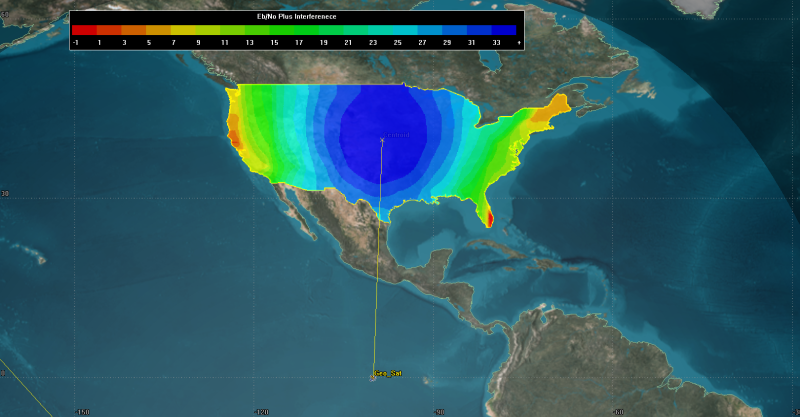
2D Graphics Coverage
Analyzing receiver interference with a Link Information Detailed report
A
- Right-click on CommSystem1 (
 ).
). - Select Report & Graph Manager... (
 ) in the shortcut menu.
 - Select the Link Information Detailed (
 ) report in the Installed Styles (
 ) folder.
 - Click .
- Scroll to the right of the report and locate the Eb/No (dB) and Eb/(No+Io) (dB) columns. The Eb/No (dB) column shows the communications without interference and the Eb/(No+Io) (dB) shows if there is interference.
- Scroll down through the report until you locate areas where the Eb/(No+Io) (dB) shows interference on the communications link. The below report is a sample custom report with the Time, Eb/No, and Eb/(No+Io).
- Close the report and the Report & Graph Manager.
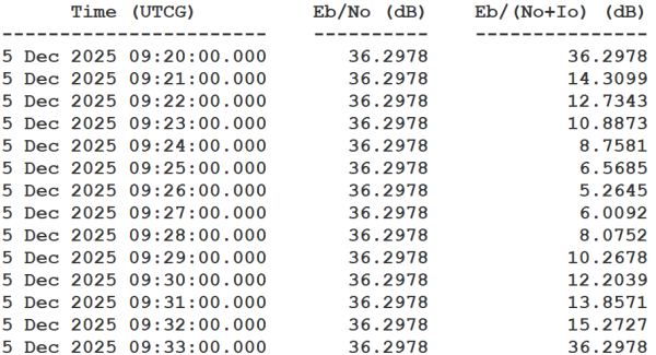
Eb/No Interference Sample
You can see from your report that there is occasional interference against DL_Rx.
Analyzing coverage interference with a Grid Stats Over Time report
A
- Right-click on EbNo_Io (
 ).
). - Select Report & Graph Manager... () in the shortcut menu.
- Select the Grid Stats Over Time () report in the Installed Styles () folder.
- Click .
- Scroll down the report until you see evidence of interference.
- Bring the 2D Graphics window to the front.
- Click Start (
 ) on the Animation toolbar to animate the scenario.
 - When finished, click Reset (
 ).
). - Close the report and the Report & Graph Manager.
The Minimum (dB) values are mostly ~ 0 dB. However, when Leo_Tx is interfering with the coverage grid, you will see those values dipping well below 0 dB.
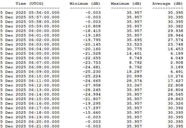
Grid Interference Sample
You will see more grid interference due to each point in the CONUS grid being evaluated instead of Centroid's receiver. The contours on the 2D and 3D Graphic windows are set for the minimum to cut off at -1 dB.
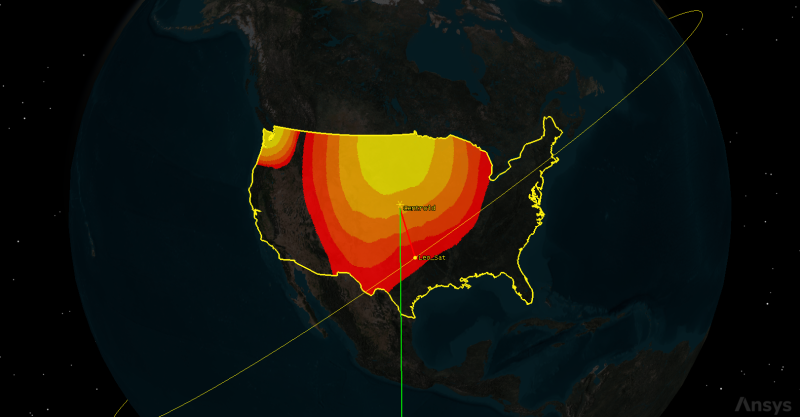
2D Graphics Interference Example
Remember, the original goal was to maintain Eb/No of approximately 0 dB across CONUS. Whenever Leo_Tx drops the Eb/No below -1 dB in the coverage grid, the contour color will disappear.
Creating a new ModelCenter project
The
- Save (
 ) your scenario.
 - Close the STK application.
- Open the ModelCenter (
 ) application.
 - Click in the Welcome to ModelCenter dialog box.
- Click when the What type of model would you like to create? dialog box opens.
- Navigate to your scenario folder (e.g. C:\Users\<username>\Documents\STK_ODTK 13\Analyzer_Interference_Analysis.
- Enter Analyzer_Interference_Analysis in the File name field.
- Ensure the Save as type is set to the ModelCenter Model (Zip) (*.pxcz).
- Click .
Configuring the STK Plugin for ModelCenter
The
- Select favorites (
 ) in the Server Browser at the bottom of the window.
 - Click and drag the STK component (
 ) into the dashed circle underneath "Drop items here to build the model" in the workflow's Analysis View.
 - Select Analyzer_Interference_Analysis.sc when the Open STK Scenario file dialog box opens.
- Click .
- After a few moments, the STK Analyzer window will open.
The Analyzer_Interference_Analysis scenario file will open in the STK application in the background.
You can add any of the STK variables as ModelCenter input or output variables through the STK Analyzer window that appears. If you change the value of a variable in your scenario through the STK interface or the ModelCenter Component Tree, you should re-add the variable into ModelCenter or re-run the workflow before running any trade studies with the new value.
Setting up your analysis with Analyzer
Use the STK Analyzer window to configure the input and output variables available for further analysis with the
Selecting the Analyzer input variables
Your studies will focus on several design specifications of the satellite's transmitter. Before you can use them in your model, however, you must first add them to your design space.
- Expand (
 ) Leo_Sat (
 ) in the STK Variables tree.
 - Select Leo_Tx (
 ).
). - Expand () the Model (Simple_Transmitter_Model) (
 ) property in the STK Property Variables tree.
 - Expand () the ModelSpecs () property.
- Select EIRP (
 ).
). - Move (
 ) EIRP () to the Analyzer Variables list as an input variable.
 - Select Frequency ().
- Move () Frequency () to the Analyzer Variables list a second input variable.
When you select an object in the STK Variables tree, all possible input variable candidates for that object are listed under the General tab and the Active Constraints tab in the STK Property Variables panel.
Note that both EIRP and Frequency are listed as Inputs in the Analyzer Variables list.
Selecting the Analyzer output variables
The same data providers that are in the Report & Graph Manager in the STK application are available in the Data Provider Variables tree.
- Expand () CONUS_Cov (
 ) in the STK variables tree.
 - Select EbNo_Io ().
- In the Data Provider Variables tree, expand () the Overall Value (
 ) data provider.
 - Move () the following data provider elements (
 ) into the Analyzer Variables list:
 - Minimum
- Maximum
- Average
- Click to confirm your selections and to close the STK Analyzer window.
Note that the variables are listed as Outputs in the Analyzer Variables list.
This will also close the STK application, which had been running in the background.
Determining the impact of EIRP on coverage
The first study you will perform plots the transmitter's EIRP against the overall coverage value of the EBNo_Io Figure of Merit.
Using the Parametric Study tool
The Parametric Study tool runs a workflow through a sweep of values for some input variable. You can plot the resulting data to view trends.
- Expand (
 ) all the elements in the Component Tree.
 - Click Parametric Study (
 ) in the Standard toolbar.
 - Click and drag EIRP (
 ) from the Component Tree to the Design Variable field when the Parametric Study tool opens.
 - Set the following Design Variable values:
- Click and drag Minimum (
 ), Maximum (), and Average () from the Component Tree to the Responses field.
 - Click .
| Option | Value |
|---|---|
| starting value | 100 |
| ending value | 10100 |
| number of samples | 11 |
Note that the step size is automatically set to 1000.
Clicking will open the Data Explorer, which is a tool used by Trade Study tools to display data while they are being collected from your Model. While data are being collected, the Data Explorer displays a progress meter, a halt button, and the data.
Creating a 2D Line Plot
Once the trade study is complete and all data have been collected, the Data Explorer toolbar becomes active. You can create plots using the Add View menu. For this study, you will create a 2D Line Plot. A 2D Line Plot displays an X-Y plot for variables in your model. Any variable in the workflow can be plotted against any other variable.
- Close the 2D Scatter Plot that opened when the trade study finished running.
- Click Add View (
 ) on the Table Page toolbar.
 - Select 2D Line Plot (
 ) in the drop-down menu.
Setting the plot variables
The chart shows Minimum vs EIRP. You could change the y dimension to Maximum or Average to adjust the plot as needed. However, you will add Maximum and Average to the plots results for comparison on one plot. Use the Plot Options menu to set which variable is displayed on which axis. In certain plots, you can set other global plot controls based on the plot variables. In this case, you want to view several variables: the minimum, maximum, and average EIRP.
- Click Dimensions in the Plot Options menu on the left-hand side of the 2D Line Plot.
- Click Add Series (+).
- Set Series 2 - x to EIRP.
- Set Series 2 - y to Maximum.
- Click Add Series (+).
- Set Series 3 - x to EIRP.
- Set Series 3 - y to Average.
- Click on the plot to close the Plot Options menu.
This adds the Maximum EIRP values to the plot.
This adds the Average EIRP values to the plot.
Setting options for the axes
Use the Axes tab to set options for the axes.
- Click Axes in the Plot Options menu.
- Select the Ticks tab.
- Change the Max # value to 20.
- Click anywhere on the plot to close the Plot Options menu.
- Review the 2D Line Plot.
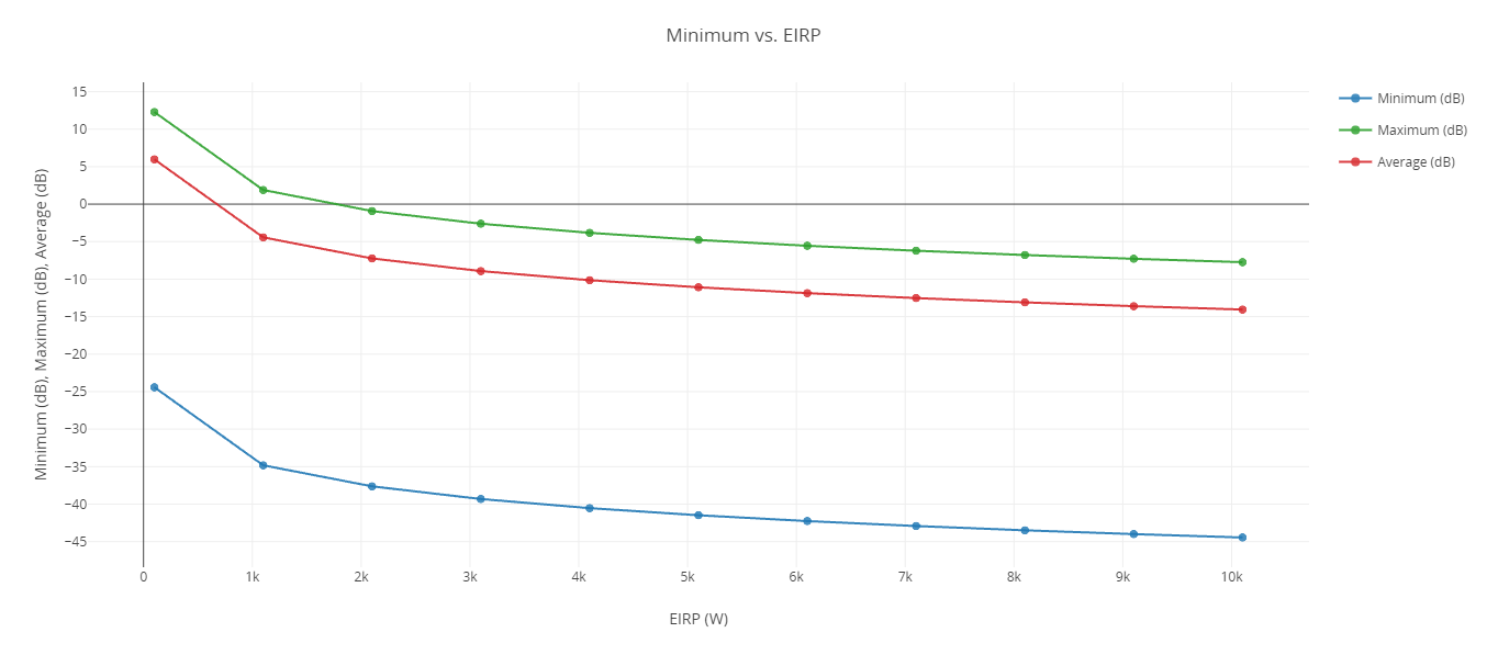
Eb/No Vs. eirp 2D Line Plot
The study shows a steep decrease in Eb/(No+Io) as the EIRP increases to about 1 kilowatt, but it begins to taper off thereafter.
Closing out your trade study
Close out your trade study for the next section.
- Close the 2D Line Plot and the Table page when you are finished.
- Click when prompted to close your trade study without saving.
Determining the impact of frequency on coverage
EIRP is not the only transmitter parameter that will impact your coverage. Frequency also has an impact.
Using the Parametric Study tool
To determine how much of an effect Frequency has on coverage, perform another Parametric Study.
- Expand () all elements in the Component Tree.
- Click and drag Frequency () from the Component Tree to the Design Variable field when the Parametric Study tool opens.
- Set the following Design Variable values:
- Click and drag Minimum (), Maximum (), and Average () from the Component Tree to the Responses field.
- Click .
This will replace EIRP as the Design Variable.
| Option | Value |
|---|---|
| starting value | 12.5 |
| ending value | 12.6 |
| number of samples | 11 |
Creating a 2D Line Plot
Create a 2D Line Plot for the study.
- Close the 2D Scatter Plot that opened when the trade study finished running.
- Click Add View () on the Table Page toolbar.
- Select 2D Line Plot () in the drop-down menu.
Setting the plot variables
The chart shows Minimum vs Frequency. Add the Maximum and Average variables to the plot's results for comparison on one plot.
- Click Dimensions in the Plot Options menu on the left-hand side of the 2D Line Plot.
- Click Add Series (+).
- Set Series 2 - x to Frequency.
- Set Series 2 - y to Maximum.
- Click Add Series (+).
- Set Series 3 - x to Frequency.
- Set Series 3 - y to Average.
- Click on the plot to close the Plot Options menu.
- Review the 2D Line Plot.
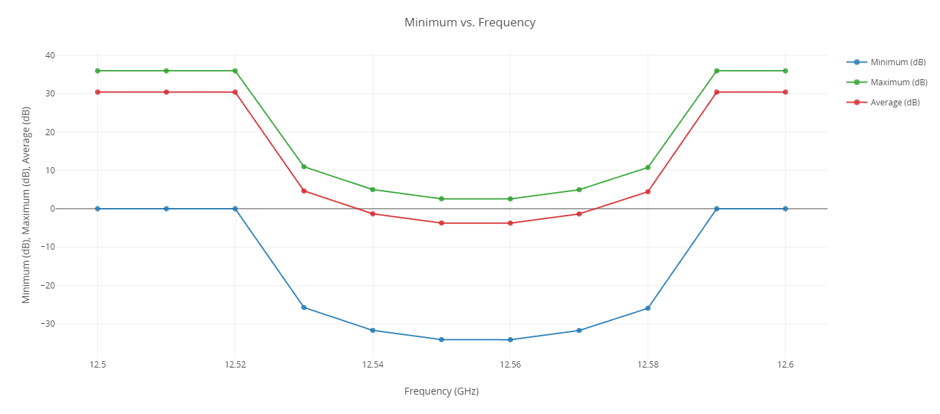
Eb/No Vs. Frequency 2D Line Plot
This study gives you an understanding of what frequency band creates the lowest overall minimum Eb/(No+Io). Eb/(No+Io) decreases with frequency as the frequency of the interferer approaches the frequency of the desired transmitter. You can see that frequencies less than 12.52 GHz and greater 12.59 GHz will assure you of an Eb/(No+Io) of approximately 0 dB for all of CONUS.
Closing out your trade study
Close out your trade study for the next section.
- Close the 2D Line Plot and the Table page when you are finished.
- Click when prompted to close your trade study without saving.
- Close the Parametric Study tool.
Determining if EIRP and frequency impact one another
You have determined that EIRP and frequency have significant impacts on coverage. This leads to the following question: How do frequency and power affect one another? You can answer the question by performing a 2-dimensional parametric study called a Carpet Plot.
Using the Carpet Plot tool
A Carpet Plot is a means of displaying data dependent on two variables in a format that makes interpretation easier than normal multiple curve plots. A Carpet Plot can be thought of as a multidimensional Parametric Study, except you now have two variables instead of one.
- Click Carpet Plot (
 ) on the Standard toolbar.
 - Click and drag Frequency () from the Component Tree to the first Design Variables field when the Carpet Plot tool opens.
- Set the following Frequency Design Variable values:
- Click and drag EIRP () from the Component Tree to the second Design Variables field.
- Set the following Frequency Design Variable values:
- Click and drag Minimum () from the Component Tree to the Responses field.
- Click .
| Option | Value |
|---|---|
| From | 12.5 |
| To | 12.6 |
| Num Steps | 3 |
| Option | Value |
|---|---|
| From | 100 |
| To | 1000 |
| Num Steps | 3 |
| Step Size | 450 |
If you are wondering why this tutorial uses large step sizes, it's due to keeping the tutorial time under an hour. These settings will require a total of nine runs to obtain every variable combination. On your own, you can set the frequencies and EIRP to change at smaller step sizes to make the trade study more realistic. Be patient. Depending on your settings, you could end up needing hundreds of runs.
Reviewing the Carpet Plot
Using the Carpet Plot, you can determine combinations of frequency and power desired which fit your requirement of an Eb/No of 0 dB.
- Review the Carpet Plot.
- Close Carpet Plot and the Table page when you are finished.
- Click when prompted to close your trade study without saving.
- Close the Carpet Plot tool.
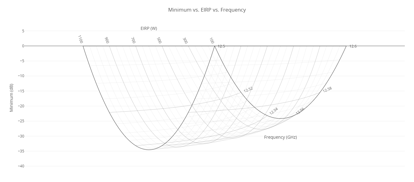
Minimum EB/No Vs. EIRP Vs. Frequency Carpet Plot
Using the Carpet Plot, basing the study on an Eb/No of 0 decibels, you can determine the combinations of frequency and EIRP that create the most interference in the coverage grid.
Saving your work
Save your work and close out ModelCenter application.
- Close out any open plots, tools, and the Data Explorer window.
- Click when prompted to close your trade study without saving.
- Click Save (
 ) to save your ModelCenter workflow.
 - Close the ModelCenter application.
Summary
You began by reviewing and visualizing the interference a satellite in low Earth orbit caused for a communications system on board a satellite in geosynchronous orbit over the contiguous United States. Using the ModelCenter application, you performed a series of parametric studies to understand the effects various transmitter and antenna design specs had on the overall EIRP of the GEO satellite's comm system. Finally, you created a carpet plot to determine the combinations of frequency and power for LEO's transmitter that created the most and least amounts of interference in the comm system.