STK Premium (Air), STK Premium (Space), or STK Enterprise
You can obtain the necessary licenses for this tutorial by contacting AGI Support at support@agi.com or 1-800-924-7244.
Required product install: The Ansys ModelCenter® model-based systems engineering software and the STK Plugin for ModelCenter are required to complete this tutorial.
ModelCenter installation prerequisites: The ModelCenter software requires the installation of a 64-bit version of Java, a 64-bit implementation of Python 3.x, and the installation of the thrift and six Python packages. See the ModelCenter Installation Prerequisites for more information.
This tutorial was written using version 2026 R1 of the Ansys ModelCenter® model-based systems engineering software.
The results of the tutorial may vary depending on the user settings and data enabled (online operations, terrain server, dynamic Earth data, etc.). It is acceptable to have different results.
Capabilities covered
This lesson covers the following capabilities of the Ansys Systems Tool Kit® (STK®) digital mission engineering software:
- STK Pro
- Radar
- STK Analyzer
- STK Analyzer Optimization
Problem statement
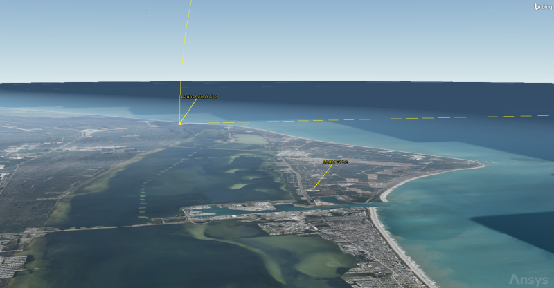
Engineers and operators want to analyze the performance of a phased-array radar system, which is used to track a launch vehicle from a site near the launch pad. You want to study the effects the input parameters of the radar have on its ability to track the launch vehicle during its ascent. In this case, the radar's performance is measured by integrated probability of detection (PDet). You want to maintain an average integrated PDet of 0.5 or above to ensure that the radar can track the launch vehicle for the greatest possible extent of its ephemeris.
Solution
Use the STK software's Radar capability and the Analyzer capability, which is part of the Ansys ModelCenter® model-based systems engineering software, to perform several parametric studies and to create a carpet plot to gain a better understanding of how the radar's wavelength and power parameters affect its performance. Then, use the STK Analyzer Optimization capability to determine the best combination of parameters that will provide the highest probability of tracking the launch vehicle.
What you will learn
Upon completion of this tutorial, you will be able to:
- Analyze a radar system for trends
- Optimize radar parameters to meet mission objectives
- Perform Parametric, Carpet Plot, and Optimization studies that vary input variables through a range of values
Using the starter scenario
To speed things up and allow you to focus on the portion of this exercise that teaches you how to use the ModelCenter software, a partially created scenario has been provided for you.
Opening the starter scenario
The starter scenario is included in your install.
- Launch the STK application (
 ).
). - Click
 Open a Scenario in the Welcome to STK dialog box.
 - Browse to <Install Dir>\Data\Resources\stktraining\VDFs.
- Select Analyzer_RadarAnalysis.vdf.
- Click .
Saving the VDF as a scenario file
Save and extract the VDF data in the form of a scenario folder. When you save a VDF in the STK application, it will save in its originating format. That is, if you open a VDF, the default save format will be a VDF (.vdf). If you want to save and extract a VDF as a scenario folder, you must change the file format by using the Save As feature. This will create a permanent scenario file complete with child objects and any additional files packaged with the VDF.
- Open the File menu when the starter scenario opens.
- Select Save As....
- Select the STK User folder in the navigation pane when the Save As dialog box opens.
- Select the Analyzer_RadarAnalysis folder.
- Click .
- Select Scenario Files (*.sc) in the Save as type drop-down list.
- Select the Analyzer_RadarAnalysis Scenario file in the file browser.
- Click .
- Click in the Confirm Save As Dialog box to overwrite the existing scenario file in the folder and to save your scenario.
A scenario folder with the same name as the VDF was created for you when you opened the VDF in the STK application. This folder contains the temporarily unpacked files from the VDF.
When saving a VDF containing external files as a scenario folder, you must extract its contents to the scenario folder the STK application automatically creates for you in the STK User folder. This allows files packaged with the VDF, such as data files, reports, presentations, HTML pages, scripts, spreadsheets, and other files, to unpack to the scenario folder. If you save the VDF as a scenario folder in another location, these additional files will not be included. See the
Save (![]() ) often during this lesson!
) often during this lesson!
LaunchVehicle and RadarSite
Defining the launch vehicle's radar cross section
You are tracking a
You will be using a custom radar cross section file to define the RCS of the launch vehicle. A file containing this data is included with the scenario. Load this file in the launch vehicle's properties.
- Right-click on LaunchVehicle (
 ) in the Object Browser.
 - Select Properties (
 ) in the shortcut menu.
 - Select the RF - Radar Cross Section page when the Properties Browser opens.
- Clear the Inherit check box at the top of the page.
- Select External File in the Compute Type field in the Band Properties Panel.
- Click the ellipsis (
 ) next to the Filename field.
 - Select the file Basic_missile_mono.rcs file in the folder and file browser when the Select File dialog box opens.
- Click to confirm your selection and to close the Select File dialog box.
- Click to confirm your changes and to close the Properties Browser.
This will allow you to set the RCS for the launch vehicle instead of it inheriting settings from the scenario level.
If you click the ellipsis (![]() ) and you're directed to a directory other than the scenario folder, browse to the scenario directory (for example, C:\Users\<username>\Documents\STK_ODTK 13\Analyzer_RadarAnalysis) and select the .rcs file.
) and you're directed to a directory other than the scenario folder, browse to the scenario directory (for example, C:\Users\<username>\Documents\STK_ODTK 13\Analyzer_RadarAnalysis) and select the .rcs file.
Computing access
You will use ModelCenter to perform studies on integrated PDet. First, you need to calculate access between the radar and launch vehicle.
- Right-click on PhasedArrayRadar (
 ).
). - Select Access... (
 ) in the shortcut menu.
 - Select LaunchVehicle () in the Associated Objects list when the Access tool opens.
- Click
 .
. - Click .
- Expand (
 ) the Installed Styles (
 ) folder in the Styles list when the Report & Graph Manager opens.
 - Select the Radar SearchTrack (
 ) report.
 - Click .
- Review the report.
- Close the Radar SearchTrack report, the Report & Graph Manager and the Access tool.
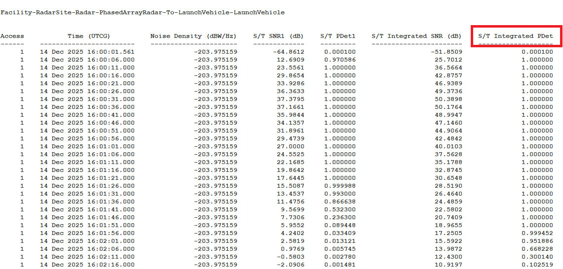
A Radar SearchTrack report provides dynamic Sear Track mode radar performance data between the radar system and the selected target.
Radar Search Track Results
Note the S/T Integrated PDet value. This value will be accessible in Analyzer as an output variable. The PDet ranges from 0.0001 to 1.0000, with the majority being below the minimum specified value of 0.5000 a little after two minutes after launch. By varying each of the parameter inputs, you'll determine which values are necessary to meet the requirement. You'll also see how a carpet plot will allow you to change more than one input at once and determine what combinations of two inputs can achieve the minimum requirement. The final optimization will provide the best combination of parameters to track the launch vehicle.
Creating a new ModelCenter project
The
- Save (
 ) your scenario.
 - Close the STK application.
- Open the ModelCenter (
 ) application.
 - Click in the Welcome to ModelCenter dialog box.
- Click when the What type of model would you like to create? dialog box opens.
- Navigate to your scenario folder (for example, C:\Users\<username>\Documents\STK_ODTK 13\Analyzer_RadarAnalysis.
- Enter Analyzer_RadarAnalysis in the File name field.
- Ensure the Save as type is set to the ModelCenter Model (Zip) (*.pxcz).
- Click .
Launching the STK Plugin for ModelCenter
The
- Select favorites (
 ) in the Server Browser at the bottom of the window.
 - Click and drag the STK component (
 ) into the dashed circle underneath "Drop items here to build the model" in the workflow's Analysis View.
 - Select Analyzer_RadarAnalysis.sc when the Open STK Scenario file dialog box opens.
- Click .
- After a few moments, the STK Analyzer window will open.
The Analyzer_RadarAnalysis scenario file will open in the STK application in the background.
You can add any of the STK variables as ModelCenter input or output variables through the STK Analyzer window that appears. If you change the value of a variable in your scenario through the STK interface or the ModelCenter Component Tree, you should re-add the variable into ModelCenter or re-run the workflow before running any trade studies with the new value.
Specifying the variables for analysis
Use the STK Analyzer window to configure the input and output variables available for further analysis with the
Selecting the Analyzer input variables
Your studies will focus on the design specifications of the radar's transmitter — specifically, the wavelength and power. Before you can use them in your model, however, you must first add them to your design space.
- Expand (
 ) RadarSite (
 ) in the STK Variables tree.
 - Select PhasedArrayRadar ().
- Expand () the SystemMonostatic (
 ) property in the STK Property Variables tree.
 - Expand () the Transmitter () property.
- Expand () the Specs () property.
- Select Wavelength (
 ).
). - Move (
 ) Wavelength () to the Analyzer Variables list.
 - Select Power ().
- Move () Power () to the Analyzer Variables list.
When you select an object in the STK Variables tree, all possible input variable candidates for that object are listed under the General tab and the Active Constraints tab in the STK Property Variables panel.
Note that both Wavelength and Power are listed under Inputs in the Analyzer variables list.
Selecting the output variables
The same data providers that are available in the Report & Graph Manager in the STK application are available in the Data Provider Variables tree.
- Expand () Access () in the STK Variables tree.
- Select Facility-RadarSite-Radar_PhasedArrayRadar-to-LaunchVehicle-LaunchVehicle (
 ).
). - At the bottom of the Data Providers list, select the Show all data providers check box.
- In the Data Providers field, expand () the Radar SearchTrack (
 ) data provider.
 - Expand () the S/T Integrated PDet (
 ) data provider element.
 - Select the Mean (
 ) statistical function.
 - Move () Mean () into the Analyzer Variables list.
- Click to confirm your selections and to close the STK Analyzer window.
Note that Mean is listed under Outputs in the Analyzer Variables list.
This will also close the STK application, which had been running in the background.
Studying the transmitter wavelength
The first parameter you will examine is the transmitter's wavelength. You need to select input and output variables from the main Analyzer window to pass to the Parametric Study tool.
Using the Parametric Study tool
The Parametric Study tool runs a workflow through a sweep of values for some input variable. You can plot the resulting data to view trends.
- Expand () all the elements in the Component Tree.
- Click Parametric Study (
 ) in the Standard toolbar.
 - Click and drag Wavelength (
 ) from the Component Tree to the Design Variable field when the Parametric Study tool opens.
 - Set the following Design Variable values:
- Click and drag Mean (
 ) from the Component Tree to the Responses field.
 - Click .
| Option | Value |
|---|---|
| starting value | 0.1 |
| ending value | 10 |
| number of samples | 51 |
| step size | 0.2 |
Clicking will open the Data Explorer, which is a tool used by Trade Study tools to display data while they are being collected from your model. While data are being collected, the Data Explorer displays a progress meter, a halt button, and the data. The Table page of the Data Explorer displays trade study data in a tabular form. It is the default window that is present for all trade studies. Cells are shaded differently depending on the associated variable's state. Input variables are shown with green text, valid values are displayed with black text, invalid values are displayed with gray text, and modified values are displayed with blue text. From the table it is possible to view and edit all values in your trade study and even to add and remove whole runs.
Creating a 2D Line Plot
Once the trade study is complete and all data have been collected, the Data Explorer toolbar becomes active. Some trade study tools will automatically launch a default plot window when the trade study runs. For other plots, you can create them from the Add View menu. For this study, you will create a 2D Line Plot. A 2D Line Plot displays an X-Y plot for variables in your model. The Data Explorer stores values for all variables in a workflow and special variables from the trade study. Any variable in the workflow can be plotted against any other variable.
- Close the 2D Scatter Plot that opened when the trade study finished running.
- Click Add View (
 ) on the Table Page toolbar.
 - Select 2D Line Plot (
 ) in the drop-down menu.
Setting options for the axes
Use the Axes tab to set options for the axes.
- Click Axes in the Plot Options menu.
- Select the Ticks tab.
- Change the Max # value to 40.
- Click the plot to close the Plot Options menu.
- Review the 2D Line Plot.
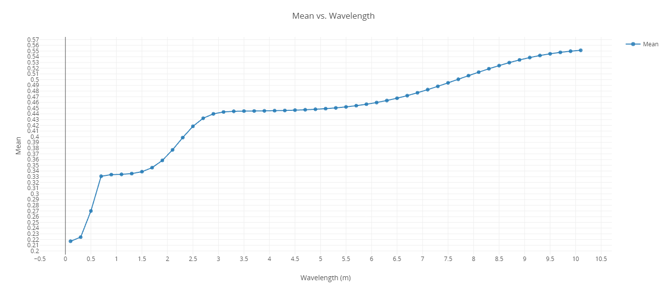
Wavelength 2D Line Plot
As the transmitter's wavelength increases (the frequency becomes lower), the average PDet increases. Between a wavelength of 3 and 6 meters, this increase tapers off.
Closing out your trade study
Close out your trade study for the next section.
- Close the 2D Line Plot and the Table page when you are finished.
- Click when prompted to close your trade study without saving.
- Leave the Parametric Study tool open.
Studying the transmitter Power
Wavelength is not the only transmitter parameter that will impact your tracking. Power also has an impact. To determine how much, run another Parametric Study.
Running the Parametric Study
Build a new Parametric Study using Power as your Design Variable.
- Click the Value field for Wavelength.
- Enter 10 for the Wavelength Value.
- Click and drag Power () from the Component Tree to the Design Variable field when the Parametric Study tool opens.
- Set the following Design Variable values:
- Click .
This will replace Wavelength as the Design variable.
| Option | Value |
|---|---|
| starting value | 100 |
| ending value | 14000 |
| number of samples | 15 |
| step size | 1000 |
Viewing the plot and adjusting the axes
After running the Parametric Study, create a line plot to view the results.
- Close the 2D Scatter Plot that opened when you ran the trade study.
- Click Add View () on the Table Page toolbar.
- Select 2D Line Plot () in the drop-down menu.
- Click Axes in the Plot Options menu.
- Select the Ticks tab.
- Change the Max # value to 20.
- Click on the plot to close the Plot Options menu.
- Review the 2D Line Plot.
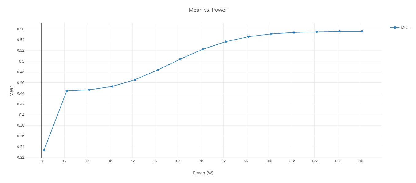
Power Change
The Power shows a steady increase of Mean Integrated PDet between 4 and 8 kW before it levels off.
Closing out your trade study
Close out your trade study for the next section.
- Close the 2D Line Plot and the Table page when you are finished.
- Click when prompted to close your trade study without saving.
- Close the Parametric Study tool.
Determining if wavelength and power impact one another
You have determined that wavelength and power have significant impacts on Integrated PDet. This leads to the following question: How do wavelength and power affect one another? You can answer the question by performing a 2-dimensional parametric study called a Carpet Plot.
Using the Carpet Plot tool
A Carpet Plot is a means of displaying data dependent on two variables in a format that makes interpretation easier than normal multiple curve plots. A Carpet Plot can be thought of as a multidimensional Parametric Study. Setting the design variables in a Carpet Plot is similar to using the Parametric Study tool except you now have two variables instead of one.
- Click Carpet Plot (
 ) on the Standard toolbar.
 - Click and drag Wavelength () from the Component Tree to the first Design Variables field when the Carpet Plot tool opens.
- Set the following Wavelength Design Variable values:
- Click and drag Power () from the Component Tree to the second Design Variables field.
- Set the following Power Design Variable values:
- Click and drag Mean () from the Component Tree to the Responses field.
- Click .
| Option | Value |
|---|---|
| From | 0.1 |
| To | 10 |
| Num Steps | 11 |
| Step Size | 1 |
| Option | Value |
|---|---|
| From | 2000 |
| To | 14000 |
| Num Steps | 13 |
| Step Size | 1000 |
If you are wondering why this tutorial uses large step sizes, it's due to keeping the tutorial time to a minimum. These settings will require a total of 143 runs to obtain every variable combination. On your own, you can set the Wavelength and Power to change at smaller step sizes to make the trade study more realistic. Be patient. Depending on your settings, you could end up running hundreds of runs.
Reviewing the Carpet Plot
Using the Carpet Plot, you can find different combinations of wavelength and power that allow you to maintain a Mean Integrated PDet of 0.5 or higher.
- Review the Carpet Plot.
- Close Carpet Plot and the Table page when you are finished.
- Click when prompted to close your trade study without saving.
- Close the Carpet Plot tool.
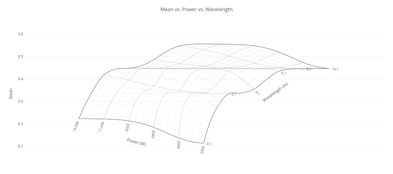
Carpet Plot
Note that the maximum Mean Integrated PDet sits around 0.55.
Optimizing the transmitter parameters
You now know that transmitter parameters have an impact on Integrated PDet. To optimize these parameters, you can either guess at values or employ an optimization tool. Although you can clearly see trends from the previous studies, guessing at values will be difficult because you are dealing with multiple parameters at the same time. To solve more complex problems, the STK Analyzer Optimization capability, by means of the ModelCenter software's Optimization tool, can be a very useful guide. The Optimization tool is a collection of optimization algorithms that you can use within the ModelCenter application. A common graphical user interface (GUI) is provided to define optimization problems. An algorithm selection wizard is also provided to make it easy to choose algorithms that will work best for the problem at hand. Use the Optimization tool to minimize the power requirement for the transmitter while maintaining an average Integrated PDet of approximately 0.5.
Creating an objective
Objective functions can be specific variables or equations composed of multiple output variables. Your objective is to minimize the value for power and maximize the Mean Integrated PDet by changing wavelength and power.
- Click Optimization Tool (
 ) in the Standard toolbar.
 - Click and drag Power () from the Component Tree to the Objective field on the right when the Optimization tool opens.
- Ensure the Goal field is set to Minimize.
- Click and drag Mean () to the Objective field.
- Open the Goal drop-down menu (
 ) for Mean.
 - Select Maximize.
Setting the constraints
Constraints restrict particular variables to a region or value.
- Click and drag Mean () to the Constraint field.
- Set the Lower Bound to 0.5.
- Set the Upper Bound to 1.0.
Selecting the Design Variables
The design variables are the variables that the optimizer will modify to meet the objective.
- Click and drag both Wavelength and () and Power () to the Design Variables field.
- Set the following Design Variable values:
| Design Variable | Start Value (Explicit Value) | Lower Bound | Upper Bound |
|---|---|---|---|
| Wavelength | 1 | 1 | 10 |
| Power | 2000 | 2000 | 14000 |
Note that each Start Value must be equal to or greater than its respective Lower Bound value.
Selecting the algorithm
Many algorithms are available, including gradient-based optimizers, genetic algorithms, multiobjective algorithms, and other heuristic search methods In this case, since you have two objectives for your study, you need to select an algorithm that can support multiple objectives.
- Open the Algorithm drop-down list.
- Select DAKOTA Multiobjective Genetic Algorithm (MOGA).
- Click .
The DAKOTA (Design Analysis Kit for Optimization and Terascale Applications) toolkit provides a flexible and extensible interface between computational models and iterative analytical methods. The MOGA algorithm uses a non-dominated algorithm to perform a Pareto search to find a set of best designs for multiobjective problems. The algorithm supports a mixture of real and discrete variables and general constraints.
While you could choose the Darwin Algorithm to perform this trade study, using it would potentially take thousands of runs and many hours to complete. Using the DAKOTA Multiobjective Genetic Algorithm will allow you to identify feasible options in only a few hundred runs.
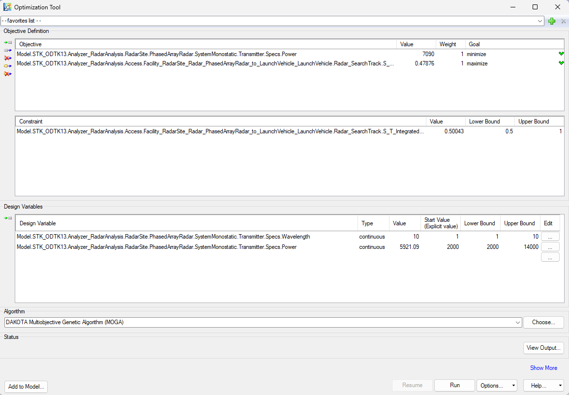
Optimization tool setup
The optimizer will display a history of steps as it progresses. By default, it will display only the objective definition.
Be patient. Your trade study may run over a period of two or more hours.
Reviewing the optimization study
The objective of your trade study is to minimize the value for power by changing wavelength and power all while maintaining an Mean Integrated PDet above a minimum of 0.5 as possible. It's possible that you won't meet your goal due to radar system limitations, but you can still get close.
- Close the 2D Scatter Plot that automatically opened after the trade study finished running.
- Return to the Optimization tool.
- Click in the Status panel to show the convergence history of the process.
- Select the Best Design tab, which contains the optimized values, when the Optimization tool Results window opens. These values are also displayed in the Value column for the design variables in the Optimization tool.
- Close the Optimization tool Results window when you are finished.
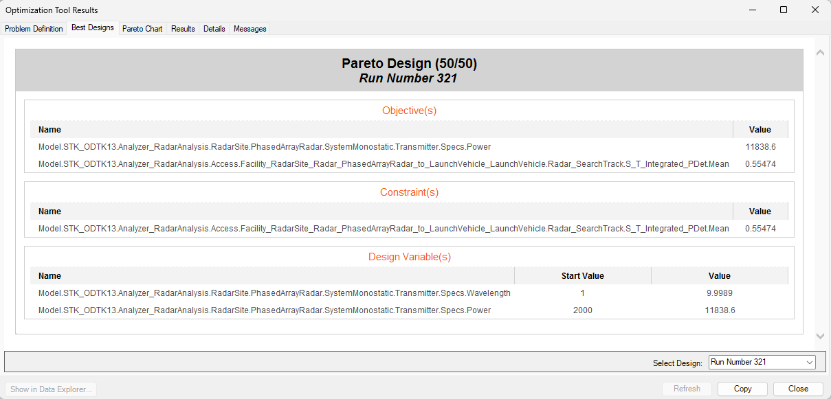
Optimization Values
You are able to maintain an average PDet above 0.5. The Optimization tool got you within the bounds.
Reviewing the optimized values
After running an optimization study, the values in your model will be changed to the final, optimized values. View the updated values.
- Return to your ModelCenter Workspace.
- Close out any open plots and the Data Explorer window.
- Click when prompted to close your trade study without saving.
- Click Save (
 ) to save your ModelCenter workflow and to keep ModelCenter open.
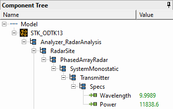
Updated values
Note the updated values of your input variables. You will need them in the next section.
Updating the values in your STK scenario
Now that your transmitter specs are optimized, update those properties in your STK scenario.
- Reopen the Analyzer_RadarAnalysis scenario in the STK application ().
- Right-click on PhasedArrayRadar ().
- Select Properties () in the shortcut menu.
- Select the Transmitter tab when the Properties Browser opens.
- Ensure the Specs sub-tab is selected.
- Enter the optimized Wavelength value in meters in the Wavelength field (for example, 9.9989 m).
- Enter the optimized Power value in Watts the Power field, rounded to one decimal point (for example, 11838.6 W).
- Click to accept your changes and to close the Property Browser.
Creating a new Radar SearchTrack report
With your radar transmitter optimized, create an new Radar SearchTrack report to view the difference.
- Right-click on PhasedArrayRadar ().
- Select Access... () in the shortcut menu.
- Click .
- Select the Radar SearchTrack () report in the My Favorites () folder in the Styles list.
- Click .
- Review the report.
- Close the Radar SearchTrack report when you are finished.
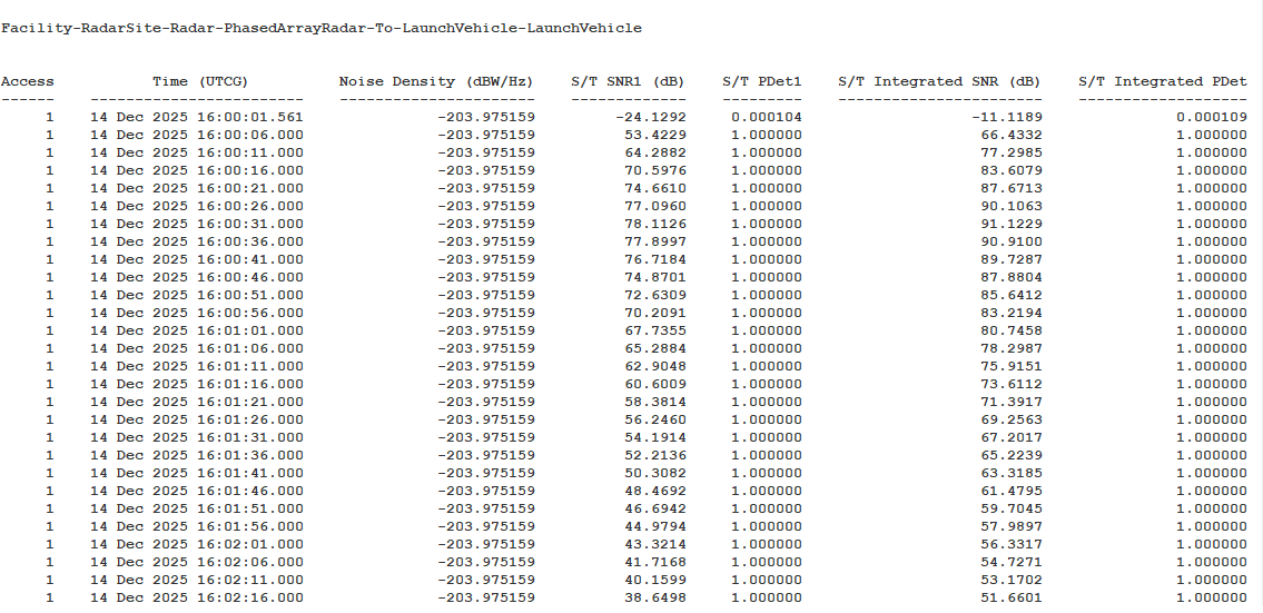
Optimized Radar SearchTrack report
You can see that with your transmitter wavelength and power optimized, you've maintained an integrated PDet of greater than 0.5 for several minutes longer than with your unoptimized radar.
Graphing the optimized radar
It can be helpful to visualize the radar search/track parameters. In this case, you'll graph the integrated signal to noise ratio (SNR) and the integrated PDet values to better understand the radar's performance.
Creating new custom graph
Create a custom graph style for Integrated PDet and SNR values over time.
- Return to the Report & Graph Manager.
- Click Create new graph style (
 ) in the Styles toolbar.
 - Enter PDet and SNR for the graph name.
- Select the Enter key.
- Expand () the Radar SearchTrack () data provider when the Graph Style window opens.
- Select the S/T Integrated SNR () data provider element.
- Move (
 ) S/T Integrated SNR () to the Y Axis list.
 - Select the S/T Integrated PDet () data provider element.
- Move () S/T Integrated PDet () to the Y2 Axis list.
- Click to accept your changes and to close the Graph Style window.
Generating the custom graph
With your custom graph configured, generate and review the data.
- Select PDet SNR (
 ) in the My Styles () folder in the Styles list.
 - Click .
- Review the graph.
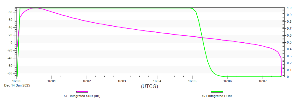
Custom S/T Integrated PDet and SNR Graph
As the launch vehicle lifts off through the beam, S/T Integrated PDet and S/T Integrated SNR rapidly rise, with S/T Integrated PDet reaching its max of 1.0 and remaining there until LaunchVehicle goes out of range. S/T Integrated SNR peaks about 30 seconds after launch (when LaunchVehicle is about 22 kilometers away) and gradually decreases from that point, although you maintain a very good SNR until the limit of the radar's range is reached.
Saving your work
Save your work and close out of the STK and ModelCenter applications.
- Close out of any open reports and tools.
- Click Save () to save your scenario.
- Close the STK application.
- Return to the ModelCenter application ().
- Close out any open plots and the Data Explorer window.
- Click when prompted to close your trade study without saving.
- Click Save () to save your ModelCenter workflow.
- Close the ModelCenter application.
Summary
You began by adding a custom RCS file to a prebuilt Launch Vehicle object. You then calculated access between a search/track radar station and the launch vehicle it was tasked with tracking using the baseline model specifications of a 0.1-meter wavelength and 40 decibel watts of power. Using the ModelCenter application, you performed a series of trade studies to understand the impact changing these model specs had on the mean integrated PDet. Using a Carpet Plot, you then analyzed the effect these variables had on each other. You then performed an optimization study to find the best frequency which would meet your design objective while minimizing the amount of power required. Finally, you updated your radar model specs in the STK application and reviewed the changes through a report and a graph.
On your own
You can conduct additional studies to optimize other parts of your radar system, including the pulse-repetition frequency (PRF), pulse width, and more. Run an additional study on the power to maximize both the Integrated PDet and Integrated SNR and review the differences between this study and optimizing for PDet alone.