STK Pro, STK Premium (Air), STK Premium (Space), or STK Enterprise
You can obtain the necessary licenses for this tutorial by contacting AGI Support at support@agi.com or 1-800-924-7244.
This lesson requires version 13.0 of the STK software or newer to complete in its entirety. If you have an earlier version of the STK software, you can complete a legacy version of this lesson.
The results of the tutorial may vary depending on the user settings and data enabled (online operations, terrain server, dynamic Earth data, etc.). It is acceptable to have different results.
Capabilities covered
This lesson covers the following capabilities of the Ansys Systems Tool Kit® (STK®) digital mission engineering software:
- STK Pro
- Communications
- Radar
Problem statement
In this lesson, you will learn how to use custom antenna and radar cross section (RCS) files to obtain a realistic simulation. You will use that simulation to analyze radio communications and radar tracking.
The lesson's scenario models how an aircrew could fly a Diamond DA-40 Diamond Star trainer aircraft from Buckley AFB to Pueblo Memorial Airport. An airport surveillance radar (ASR) is located at the City of Colorado Springs Municipal Airport and will track the aircraft. Controllers located at Pueblo Memorial Airport will establish voice communications with the aircraft prior to landing. You want to determine when controllers can track and communicate with the aircraft.
Solution
Use the STK software's Communications and Radar capabilities with antenna pattern and RCS files produced using the Ansys HFSS™ high-frequency electromagnetic simulation software, which is a part of the Ansys Electronics Desktop (AEDT)™ electronics systems design platform, to simulate the scenario.
What you will learn
When you complete the scenario, you will know:
- When the ASR system can track the small aircraft
- When air traffic controllers can communicate with the aircrew
Based on the STK software capabilities you will use, you will have:
- A basic understanding of how to use external Ansys HFSS-generated antenna and RCS files in the STK application
- Knowledge of the data contained in the HFSS-generated files
Video guidance
Watch the following video. Then follow the steps below, which incorporate the systems and missions you work on (sample inputs provided).
Downloading the required starter scenario
A partially created scenario has been created for you so you can focus on the portion of this lesson about Ansys HFSS-generated files with the STK software. The scenario is saved as a visual data file (VDF).
- Download the zipped folder here: https://support.agi.com/download/?type=training&dir=sdf/help&file=STK_and_HFSS_v13.zip
If you are not already logged in, you will be prompted to log in to agi.com to download the file. If you do not have an agi.com account, you will need to create one. The user approval process can take up to three (3) business days. Please contact support@agi.com if you need access sooner.
- Navigate to the downloaded folder.
- Right-click on STK_and_HFSS_v13.zip.
- Select Extract All... in the shortcut menu.
- Set the Files will be extracted to this folder: path to the location of your choice. The default path is C:\Users\<username>\Downloads\STK_and_HFSS_v13).
- Click .
- Go to the chosen folder.
- STK_and_HFSS.vdf will be in the extracted folder.
Opening the starter scenario
Open the downloaded scenario.
- Launch the STK application (
 ).
). - Click Open a Scenario
 in the Welcome to STK dialog box.
 - Browse to location of your extracted VDF file.
- Select STK_and_HFSS.vdf.
- Click .
Saving the VDF as a scenario
Save and extract the VDF data in the form of a scenario folder. When you save a VDF in the STK application, it will save in its originating format. That is, if you open a VDF, the default save format will be a VDF (.vdf). If you want to save and extract a VDF as a scenario folder, you must change the file format by using the Save As feature. This will create a permanent scenario file complete with child objects and any additional files packaged with the VDF.
- Open the File menu.
- Select Save As....
- Select the STK User folder in the navigation pane when the Save As dialog box opens.
- Select the STK_and_HFSS folder.
- Click .
- Select Scenario Files (*.sc) in the Save as type drop-down list.
- Click .
- Click in the Confirm Save As dialog box to overwrite the existing scenario file in the folder and to save your scenario.
- The following Ansys HFSS CSV files will be extracted to the STK_and_HFSS folder:
- MD4-200_H_Incident_2p8GHz.csv
- MD4-200_V_Incident_2p8GHz.csv
A scenario folder with the same name as the VDF was created for you when you opened the VDF in the STK application. This folder contains the temporarily unpacked files from the VDF.
When saving a VDF containing external files as a scenario folder, you must extract its contents to the scenario folder the STK application automatically creates for you in the STK User folder. This allows files packaged with the VDF, such as data files, reports, presentations, HTML pages, scripts, spreadsheets, and other files, to unpack to the scenario folder. If you save the VDF as a scenario folder in another location, these additional files will not be included. See the
Save (![]() ) often during this scenario!
) often during this scenario!
Understanding the starter scenario
Prior to modifying the scenario, you should become familiar with the objects already created in the starter scenario.
- Bring the 2D Graphics window to the front.
- Look at the flight route of the aircraft.
The aircraft's flight route starts at an altitude of 1,000 feet near Buckley AFB, climbs to 10,000 feet while passing over the Black Forrest VORTAC navaid, and then descends to 1,000 feet as it approaches Pueblo Memorial Airport. An air surveillance radar is located at the City Of Colorado Springs Municipal Airport which will track the aircraft. Air traffic controllers are located at Pueblo Memorial Airport. They will establish communications with the trainer aircraft.
If you want to know more about how exactly to create a flight route in the STK software, check out the Level 1 STK training lessons to learn all of the STK software's fundamental features.
In this scenario, you are not using visual or analytical terrain. You are using the WGS84 for altitude reference. The Aircraft object is using the Great Arc Propagator.
Ansys HFSS SBR+ radar cross section files
The radar cross section (RCS) is the measure of a target's ability to reflect radar signals in the direction of the radar receiver. Efficient modeling of the RCS with the
Each run in the HFSS software produces results for one signal source polarization. For example, a signal source model with horizontal (H) polarization computes RCS returns for the H-H (H incident and H reflected signal polarization) combination and for V-H (H incident and V reflected signal polarization). V is the vertical polarization. A second run produces data for V signal polarization and computes RCS returns for the V-V (V incident and V reflected signal polarization) combination and for H-V (V incident and H reflected signal polarization).
Using the Ansys HFSS CSV file format with the STK software
The STK software can use each data file independently when processing single polarization type. However, you can combine the exported files to produce a Complex Scattering RCS Matrix for [HH, HV, VH, VV] RCS Values. The STK software reads the column headers in the CSV format files and parses the data in each column: the RCS data frequency value, the polarization scattering matrix element (H-H, V-H, H-V, V-V), Phi angle start value (degrees), and Phi angle stop value. The STK software then computes the Phi angle step value. The first column of the CSV file represents the theta angle values. Each row corresponds to the RCS data row in the scattering matrix. The starting, ending, and step size for the theta values are determined by reading the first column data.
The following conditions apply:
- The scattering matrix data is expected to conform to a polar coordinate frame with uniform step size for Theta and Phi angles.
- The RCS data reference axis is the X-axis of the target body.
- If you use two files to import the full scattering matrix, the two files must have the same matrix size, Theta angles, Phi angles, and step size.
- The frequency values listed in the two RCS data files must be same.
Viewing the CSV files' contents
You can view the two example sample files for 2.8GHz, one for H_Incident and one for V_Incident.
- Open Windows File Explorer.
- Browse to your scenario folder (e.g. C:\Users\<username>\Documents\STK_ODTK 13\ STK_and_HFSS).
- Right-click on MD4-200_H_Incident_2p8GHz.csv.
- Select Open.
- Close (
 ) the MD4-200_H_Incident_2p8GHz.csv file.
 - Return to your scenario folder.
- Right-click on MD4-200_V_Incident_2p8GHz.csv.
- Select Open.
- Close () the MD4-200_V_Incident_2p8GHz.csv file and Windows File Explorer when finished.
- Return to the STK application.
The first column represents the theta values. The column header row (first row of the CSV file) shows the polarization, the frequency values, and the Phi angle values. The data in column two and beyond are complex RCS data values in the format a + bi.
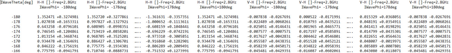
H_Incident sample

V_Incident sample
Using the Ansys HFSS files for analysis
Configuring your aircraft's properties to use Ansys HFSS CSV files for analysis
You need to configure the Aircraft object's properties so that you can use the Ansys HFSS CSV files analytically.
- Right-click on DA_40 (
 ) in the Object Browser.
 - Select Properties (
 ).
). - Select the RF - Radar Cross Section page.
- Clear the Inherit check box.
- Select Ansys HFSS CSV File from the Compute Type drop-down in the Band Properties panel.
This enables you to set the RCS settings for the Aircraft (![]() ) object instead of inheriting the settings from the Scenario (
) object instead of inheriting the settings from the Scenario (![]() ) object.
) object.
Loading the H Incident Ansys HFSS CSV file for analysis
You will use a nominal H incident Ansys HFSS CSV file that is provided for your analysis.
- Click the Primary Pol File ellipsis (
 ).
). - Click .
- Select your scenario folder.
- Click .
- Select MD4-200_H_Incident_2p8GHz.csv.
- Click .
Loading the V Incident Ansys HFSS CSV file for analysis
You will use a nominal V incident Ansys HFSS CSV file that is provided for your analysis.
- Click the Ortho Pol File ellipsis ().
- Click .
- Select your scenario folder.
- Click .
- Select MD4-200_V_Incident_2p8GHz.csv
- Click .
- Click to accept your changes and keep the Properties Browser open.
Visualizing the radar cross section in the 3D Graphics window
Update the Aircraft object's RCS settings, so you can view it in the 3D Graphics window on the
- Select the 3D Graphics - Radar Cross Section page.
- Select the Show Volume check box in the Volume Graphics panel.
- Set the following:
- Click to accept your changes and close the Properties Browser.
| Option | Value |
|---|---|
| Show as wireframe | Selected |
| Scale (per dBsm) | 2 m |
| Minimum Displayed RCS | -10 dB |
| Set theta and rho resolution together | Selected |
| Theta - Resolution | 0.5 deg |
Viewing the RCS in the 3D Graphics window
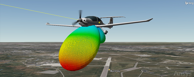
Look at the RCS in the 3D Graphics window.
- Right-click on DA_40 () in the Object Browser.
- Select Zoom To.
- Bring the 3D Graphics window to the front.
- Use your mouse to object a good view of the aircraft and its RCS.

3D Graphics View of the RCS
Inserting the radar antenna servo system
You will insert a Sensor object to simulate a servo system for radar antenna positioning. You will lock the sensor onto the aircraft and constrain the sensor to point in a limited area.
- Select Sensor (
 ) in the Insert STK Objects tool.
 - Select the Insert Default () method.
- Click .
- Select COS_Radar (
 ) in the Select Object dialog box.
 - Click .
- Right click on Sensor1 () in the Object Browser.
- Select Rename in the shortcut menu.
- Rename Sensor1 () to Servo_System.
Defining the sensor field of view
You will define Servo_System's field of view using a Simple Conic sensor pattern. You will use the sensor's field of view for situational awareness when Servo_System points the radar antenna at DA_40.
- Open Servo_System's () Properties ().
- Select the Basic - Definition page.
- Enter 1 deg in the Cone Half Angle field in the Simple Conic panel.
- Click .
Targeting the aircraft
You will use the Targeted pointing type to point Servo_System to DA_40.
- Select the Basic - Pointing page.
- Select Targeted as the Pointing Type.
- Move (
 ) DA_40 () from the Available Targets list to the Assigned Targets list.
 - Click .
Setting elevation angle and range constraints
There are many types of radar systems. A typical airport surveillance radar's nominal range is 60 miles and the elevation angle of the beam can track from 0 to 30 degrees. Anything higher than 30 degrees is the cone of silence in which the radar cannot track the aircraft. Extend Servo_System's (![]() ) maximum range further than 60 miles in order to lock onto the aircraft when it's above the horizon.
) maximum range further than 60 miles in order to lock onto the aircraft when it's above the horizon.
Adding elevation angle and range constraints to the Active Constraints list
- Select the Constraints - Active page.
- Click Add new constraints (
 ) in the Active Constraints toolbar.
 - Enter Elevation Angle in the Search field when the Select Constraints to Add dialog box opens.
- Select Elevation Angle in the Constraint Name list.
- Click .
- Enter Range in the Search field.
- Select Range in the Constraint Name list.
- Click .
- Click to close the Select Constraints to Add dialog box.
Setting the elevation angle and range constraints
- Select Elevation Angle in the Active Constraints list.
- Keep the Min check box selected in the Elevation Angle panel.
- Select the Max check box in the Elevation Angle panel.
- Enter 30 deg in Max field.
- Select Range in the Active Constraints list.
- Keep the Min check box selected in the Range panel.
- Select the Max check box in the Range panel.
- Enter 150 km in the Max field.
- Click .
Modeling an airport surveillance radar
Inserting an airport surveillance radar
You will insert a Radar object to create an airport surveillance radar. You will model actual airport surveillance radar specifications that are easily available to the public.
- Insert a Radar (
 ) object using the Insert Default () method.
 - Select Servo_System () in the Select Object dialog box.
- Click .
- Rename Radar1 () to ASR.
Modeling a monostatic radar
You will model a Monostatic radar with a Search/Track mode. This model resembles a common antenna for transmitting and receiving, along with detecting and tracking point targets.
- Open ASR's () Properties ().
- Select the Basic - Definition page.
- Notice Radar System defaults to Monostatic.
- Select the Mode tab.
- Notice Radar Monostatic Mode defaults to Search Track.
Defining the waveform
The waveform in your system will use a fixed pulse repetition frequency (PRF), with a PRF of 1000 Hz (approximately). Radar systems often use multiple pulse integration to increase the signal-to-noise ratio. The PRF is the number of pulses of a repeating signal in a specific time unit. After producing a brief transmission pulse, the transmitter is turned off in order for the receiver to hear the reflections of that signal off of targets.
- Select the Pulse Definition sub-sub-tab.
- Notice Waveform defaults to Fixed PRF.
- Notice PRF defaults to 0.001 MHz (1000 Hz).
Defining the pulse width
Pulse width is the width of the transmitted pulse (the uncompressed RF bandwidth is the inverse of the pulse width). Set the pulse width to one microsecond.
- Open the Pulse Width units (
 ) shortcut menu.
 - Select usec.
- Enter 1 usec in the Pulse Width field.
- Click .
Defining the antenna pattern
You can model the antenna using the cosine squared aperture rectangular antenna pattern. The antenna transmit frequency for this radar is between 2.7-2.9 GHz.
- Select the Antenna tab.
- Select the Model Specs sub-tab.
- Click the Antenna Model Component Selector ().
- Select the Cosine Squared Aperture Rectangular (
 ) in Antenna Model list when the Select Component dialog box opens.
 - Click to close the Select Component dialog box.
Setting the Cosine Squared Aperture Rectangular Antenna Model's properties
Set the cosine squared aperture rectangular antenna model's properties.
- Select the Use Beamwidth option.
- Set the following:
- Click .
| Option | Value |
|---|---|
| X Dim Beamwidth | 5 deg |
| Y Dim Beamwidth | 1.4 deg |
| Design Frequency | 2.8 GHz |
| Main-lobe Gain | 34 dB |
| Efficiency | 55 % |
Defining the radar transmitter
The transmitter has a frequency range of 2.7-2.9 GHz and a peak power of 25 kW.
- Select the Transmitter tab.
- Select the Specs sub-tab.
- Select the Frequency option.
- Enter 2.8 GHz in the Frequency field.
- Enter 25 kW in Power field.
- Click .
Computing the probability of detection
You will base the probability of detection (Pdet) on a value of 0.800000 or higher with one as the highest value.
- Right-click on ASR () in the Object Browser.
- Select Access... (
 ) in the shortcut menu.
 - Select DA_40 () in the Associated Objects list when the Access Tool opens.
- Click
 .
.
Generating a Radar SearchTrack report
Now that you calculated Access between ASR (![]() ) and DA_40 (
) and DA_40 (![]() ), you will generate a Radar SearchTrack report.
), you will generate a Radar SearchTrack report.
- Click under the Reports panel.
- Select the Radar SearchTrack report (
 ) in the Installed Styles list.
 - Click
Determining SearchTrack integrated probability of detection
Look at S/T Integrated Pdet in the report. S/T Integrated PDet uses multiple pulses.
- Look at the first line in the report.
- Locate the S/T Integrated Pdet column.
- Locate the S/T Pulses Integrated column.
- Scroll down the report. Pulse integration improves the ability of the radar to detect targets by combining the returns from multiple pulses which you can see in the S/T Pulses Integrated column.
- Notice that overall tracking is good.
- Close the report, the Report & Graph Manager, and the Access tool when finished.
You can track the trainer aircraft for approximately 14 minutes.
Cleaning up your scenario
Next, you will determine communications between the trainer aircraft and air traffic controllers at Pueblo Memorial Airport. Turn off all 3D Graphic visuals for the RCS and the radar servo system.
- Open DA_40's () Properties ().
- Select the 3D Graphics - Radar Cross Section page.
- Clear the Show Volume check box in the Volume Graphics panel.
- Click .
- Clear the Servo_System () check box in the Object Browser.
Exploring Ansys HFSS Far Field Data (.ffd) files
You can define a Far Field Incident Wave Source as a plain text data file with a .ffd suffix. The source can be dependent on the frequency. You will use a nominal frequency dependent Far Field Data file (.ffd) that is provided for your analysis. This .ffd file simulates a nominal blade antenna that has a design frequency of 1.2 GHz and was designed and created using the Ansys HFSS software.
- Open Windows File Explorer.
- Browse to your scenario folder (e.g. C:\Users\<username>\Documents\STK_ODTK 13\STK_and_HFSS).
- Right-click on Blade_Antenna.ffd.
- Select Open With.
- Select Notepad in the Apps list.
- Compare your .ffd file with the following format. For frequency-dependent far field links, the data is supplied in blocks. The syntax for a frequency-dependent far field uses this format.
- Close () the Blade_Antenna.ffd file and Windows File Explorer.
ThetaStart ThetaStop ThetaNumPoints
PhiStart PhiStop PhiNumPoints
Frequencies NumFrequencies
Frequency FrequencyValue
E_theta_real E_theta_imag E_phi_real E_phi_imag
E_theta_real E_theta_imag E_phi_real E_phi_imag
E_theta_real E_theta_imag E_phi_real E_phi_imag
… repeat for all theta and phi sweep points
Frequency FrequencyValue
E_theta_real E_theta_imag E_phi_real E_phi_imag
E_theta_real E_theta_imag E_phi_real E_phi_imag
E_theta_real E_theta_imag E_phi_real E_phi_imag

… repeat for all theta and phi sweep points
… repeat for a total of NumFrequencies
Building your aircraft receiver
You will attach a Receiver (![]() ) object to your trainer aircraft.
) object to your trainer aircraft.
- Insert a Receiver (
 ) object using the Insert Default () method.
 - Select DA_40 () in the Select Object dialog box.
- Click .
- Rename Receiver1 () to Acft_Rx.
Using a complex receiver
You need to use a complex receiver model so that you can use the Ansys ffd formatted antenna pattern.
- Open Acft_Rx's () Properties ().
- Select the Basic - Definition page.
- Click the Receiver Model Component Selector ().
- Select Complex Receiver Model () in the Receiver Models list in the Select Component dialog box.
- Click to close the Select Component dialog box.
- Click .
Using the ANSYS ffd Format for the antenna
Changing the antenna model to the ANSYS ffd Format
You will change your antenna model to the ANSYS ffd Format.
- Select the Antenna tab.
- Select the Model Specs sub-tab.
- Click the Antenna Model Component Selector ().
- Select ANSYS ffd Format () in the Antenna Models list in the Select Component dialog box.
- Click to close the Select Component dialog box.
Importing the Blade_Antenna.ffd file
You will import the Blade_Antenna.ffd file that is provided for your analysis.
- Click the External Filename ellipsis ().
- Click .
- Select your scenario folder.
- Click .
- Select Blade_Antenna.ffd.
- Click .
- Click .
Visualizing the antenna pattern in the 3D Graphics window
Update the receiver object's properties, so you can view the antenna pattern in the 3D Graphics window.
- Select the 3D Graphics - Attributes page.
- Select the Show Volume check box in the Volume Graphics panel.
- Set the following:
- Click .
| Option | Value |
|---|---|
| Show as wireframe | Selected |
| Gain Scale (per dB) | 2 m |
| Minimum Displayed Gain | -20 dB |
| Set azimuth and elevation resolution together | Selected |
| Azimuth - Resolution | 0.5 deg |
Viewing the antenna pattern in the 3D Graphics window
View the antenna pattern in the 3D Graphics window.
- Right-click on DA_40 in () the Object Browser.
- Select Zoom To.
- Bring the 3D Graphics window to the front.
- Use your mouse to get a good view of the aircraft and the receiver antenna pattern.

3D Graphics Antenna Pattern
Reorienting the antenna pattern
You need to orient the antenna pattern correctly. Reorient the antenna pattern 90 deg.
- Return to Acft_Rx's () Properties ().
- Select the Basic - Definition page.
- Select the Antenna tab.
- Select the Orientation sub-tab.
- Enter 90 deg in the Azimuth field.
- Click .
Viewing the antenna pattern in the 3D Graphics window
View the antenna's updated orientation in the 3D Graphics window.
- Bring the 3D Graphics window to the front.
properly oriented antenna pattern
The antenna pattern is properly aligned. This is a good example of using 3D Graphics - Attributes to help you visualize potential problems with your setup.
Inserting the Pueblo Memorial Airport Transmitter
You can insert a Transmitter object at IFS_Pueblo.
- Insert a Transmitter (
 ) object using the Insert Default () method.
 - Select IFS_Pueblo () in the Select Object window.
- Click .
- Rename Transmitter1 () to Pueblo_Tx.
Using the default simple transmitter model
A simple transmitter model uses an isotropic antenna.
- Open Pueblo_Tx's () Properties ().
- Select the Basic - Definition page.
- Notice the Simple Transmitter Model is selected by default.
- Set the following:
- Click .
| Option | Value |
|---|---|
| Frequency: | 1.2 GHz |
| Data Rate: | 1 Mb/sec |
Computing carrier to noise ratio (C/N)
Determine an effective carrier to noise ratio (C/N) focusing on voice communications.
- Right-click Acft_Rx () in the Object Browser.
- Select Access... ().
- Expand (
 ) IFS_Pueblo () in the Associated Objects list.
 - Select Pueblo_Tx ().
- Click .
Using a Link Budget to finish the mission
Based on the receiver's capabilities, you want a C/N of 15 dB or higher.
- Click in the Reports panel.
- Locate the C/N (dB) column in the Link Budget report.
- Scroll down.
You have effective voice communications between the aircraft and the air traffic controller for approximately 23 minutes.
Saving your work
- Close any properties, reports, and the Access Tool.
- Save (
 ) your work.
Summary
In this lesson, you focused on analyzing an aircraft RCS using Ansys HFSS .csv files and analyzing a link budget using an Ansys HFSS .ffd blade antenna. You applied this analysis to determine how the ASR system can track the small aircraft and when air traffic controllers can communicate with the aircrew.
If you want to know more about radar and communication design, you can learn more in the Level 1 STK training lessons. Also, you can learn more online about the Ansys HFSS software.