STK Premium (Air) and STK Premium (Space) or STK Enterprise
You can obtain the necessary licenses for this tutorial by contacting AGI Support at support@agi.com or 1-800-924-7244.
This lesson requires STK 13.0 or newer to complete in its entirety. If you have an earlier version of the STK software, you can view a legacy version of this lesson.
The results of the tutorial may vary depending on the user settings and data enabled (online operations, terrain server, dynamic Earth data, etc.). It is acceptable to have different results.
Capabilities covered
This lesson covers the following capabilities of the Ansys Systems Tool Kit® (STK®) digital mission engineering software:
- STK Pro
- Communications
- STK SatPro
Problem statement
Across the industry, the digital engineering process is becoming more complex. Systems of systems are changing and updating in different stages of the mission life cycle. In this series, you will address these challenges by creating a fully connected digital thread with a common mission environment at the core. You will design and test a new satellite constellation for persistent stereo coverage of hypersonic vehicles across the world. You will address this topic in stages: satellite constellations, hypersonic flight, EOIR sensors, communications links, and triggering events and systems. The vision is to integrate the mission environment and operational objectives into the digital thread early and throughout the entire product life cycle. Through digital mission engineering, you are now capable of quickly evaluating the overall mission impact of the smallest change to any component. This session will focus on creating a communications system. This communications system will be an important factor in the system response time of a detection and tracking system. After you figure out how well your communications system works and which satellites are doing the communicating, you will look at the system response time of the mission as a whole in the next part of the Digital Mission Engineering (DME) series.
Solution
Using the same models constructed through the design phase, you will evaluate relationships between assets like communications link availability and determine which satellites in a constellation of satellites can talk to a ground terminal during the flight of the X-43 Hyper-X Research Vehicle (HXRV).
What you will learn
Upon completion of this tutorial, you will be able to:
- Build and analyze a communications link
- Use external antenna gain pattern files
- Generate a Link Budget
Video guidance
Watch the following video. Then follow the steps below, which incorporate the systems and missions you work on (sample inputs provided).
Downloading the required starter scenario
A partially created scenario containing the X-43's test flight has been provided for you. The scenario is saved as a visual data file (VDF).
- Download the zipped folder here: https://support.agi.com/download/?type=training&dir=sdf/help&file=DME_Session3_Starter_Comms_v13.zip
If you are not already logged in, you will be prompted to log in to agi.com to download the file. If you do not have an agi.com account, you will need to create one. The user approval process can take up to three (3) business days. Please contact support@agi.com if you need access sooner.
- Navigate to the downloaded folder.
- Right-click on DME_Session3_Starter_Comms_v13.zip.
- Select Extract All... in the shortcut menu.
- Set the Files will be extracted to this folder: path to the location of your choice. The default path is C:\Users\<username>\Downloads\DME_Session3_Starter_Comms_v13).
- Click .
- Go to the chosen folder.
- DME_Session3_Starter_Comms.vdf will be in the extracted folder.
Opening the starter scenario
Open the downloaded scenario in the STK application.
- Launch the STK application (
 ).
). - Click Open a Scenario (
 ) in the Welcome to STK dialog box.
 - Browse to location of your extracted VDF file.
- Select DME_Session3_Starter_Comms.vdf.
- Click .
Saving the VDF as a scenario
Save and extract the VDF data in the form of a scenario folder. When you save a VDF in the STK application, it will save in its originating format. That is, if you open a VDF, the default save format will be a VDF (.vdf). If you want to save and extract a VDF as a scenario folder, you must change the file format by using the Save As feature. This will create a permanent scenario file complete with child objects and any additional files packaged with the VDF.
- Open the File menu.
- Select Save As....
- Select the STK User folder in the navigation pane when the Save As dialog box opens.
- Select the DME_Session3_Starter_Comms folder.
- Click .
- Select Scenario Files (*.sc) as the Save as type.
- Select the DME_Session3_Starter_Comms Scenario file in the file browser.
- Click .
- Click when the Confirm Save As dialog box opens to overwrite the existing scenario file in the folder and to save your scenario.
- The following files will be extracted to the DME_Session3_Starter_Comms folder:
- SatCom_Omni_2p2G_Installed.pattern: This is a simple antenna pattern model file you will load into the scenario.
- SatCom_Omni_2p2G_Isolation.pattern: This is an antenna pattern model file created using the
A folder with the same name as the VDF was created for you when you opened the VDF in the STK application. This folder contains the temporarily unpacked files from the VDF.
When saving a VDF containing external files as a scenario folder, you must extract its contents to the scenario folder the STK application automatically creates for you in the STK User folder. This allows files packaged with the VDF, such as data files, reports, presentations, HTML pages, scripts, spreadsheets, and other files, to unpack to the scenario folder. If you save the VDF as a scenario folder in another location, these additional files will not be included. See the
Save (![]() ) often during this lesson!
) often during this lesson!
Modeling the communications ground terminal
You will begin building your communications system by creating a ground terminal. The ground terminal houses a receiver.
Inserting a Facility object
Use a
- Bring the Insert STK Objects tool (
 ) to the front.
 - Select Facility (
 ) in the Scenario Objects list.
 - Select the Define Properties (
 ) method.
 - Click .
- Select the Basic - Position page in the Properties Browser.
Setting the ground terminal's location
Update the ground terminal's properties to place it at the correct location.
- Set the following options in the Position panel:
- Click to accept your changes and to close the Properties Browser.
- Right-click on Facility1 () in the Object Browser.
- Select Rename in the shortcut menu.
- Rename Facility1 () GroundTerminal.
| Option | Value |
|---|---|
| Latitude | 34.1084 deg |
| Longitude | -119.065 deg |
Viewing the ground terminal in the 3D Graphics window
Gain situational awareness by viewing the ground terminal's location on Laguna Peak, near Naval Base Ventura County - Point Mugu.
- Bring the 3D Graphics window to the front.
- Right-click on GroundTerminal () in the Object Browser.
- Select Zoom To in the shortcut menu.
- Move around in the 3D Graphics window to understand the location of the ground terminal.
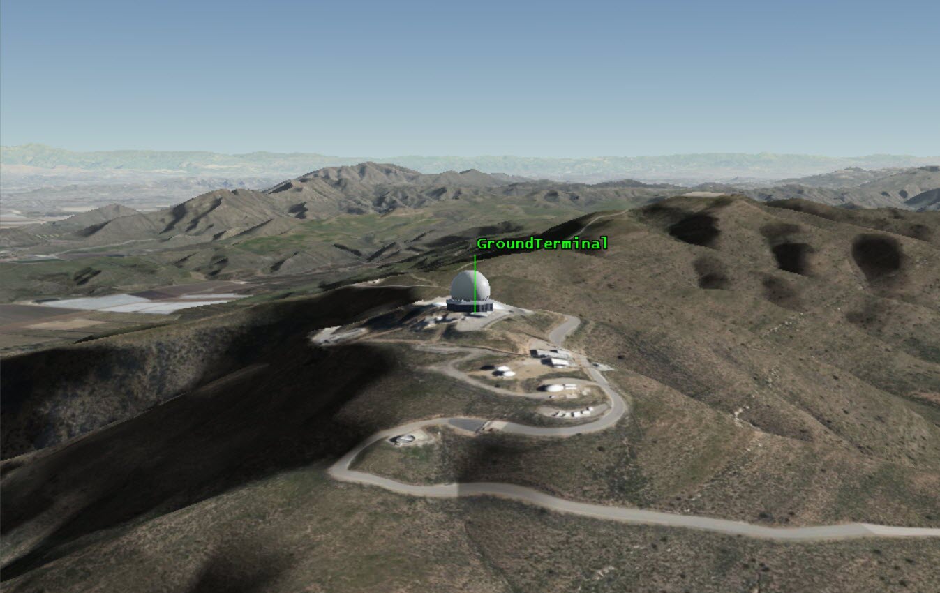
3D Graphics View of GroundTerminal
Inserting a Receiver object
Attach a
- Insert an Receiver (
 ) object using the Insert Default () method.
 - Select GroundTerminal () in the Select Object dialog box.
- Click .
- Rename Receiver1 () Receiver.
Modeling a communications satellite
The satellite collection communicates with the ground terminal receiver. Use a single Satellite object to compare the coverage between antenna models. It also functions as a seed satellite for a satellite collection you will set up later.
Inserting a Satellite object
A
- Insert a Satellite (
 ) object using the
  ) method.
 - Set the following options in the Orbit Wizard:
| Option | Value |
|---|---|
| Type | Circular |
| Satellite Name | LEO_Sat |
| Inclination | 50 deg |
| Altitude | 1734 km |
The orbital values were found from another optimization of the satellite constellation. After the initial study in the
Updating the satellite's 3D model
Change the satellite's 3D model to more close visualize a satellite that is part of the Space Tracking and Surveillance System, which your satellite collection will model. This 3D model was also used in the Ansys HFSS software to model the antenna patterns used later in this lesson.
- Click the 3D Model ellipsis (
 ) in the Graphics panel.
 - Select stss.glb in the File dialog box.
- Click .
- Click to close the Orbit Wizard.
Inserting a Transmitter object
Attach a
- Insert a Transmitter (
 ) object using the Define Properties () method.
 - Select LEO_Sat () in the Select Object dialog box.
- Click .
Defining the transmitter model
You can now begin building the communications system. Initially, you want to model a simple, omnidirectional transmitter and analyze the communications link. The default
- Select the Basic - Definition page in the Properties Browser.
- Select the Model Specs tab.
- Enter 2.2 GHz in the Frequency field. This is a short range S-Band frequency.
- Click to accept your changes and to close the Properties Browser.
- Rename Transmitter1 () Transmitter.
Generating a Link Budget to the ground terminal
Create a Link Budget report using the simple transmitter model, then update it with a unique antenna pattern.
- Right-click on Transmitter () in the Object Browser.
- Select Access... (
 ) in the shortcut menu.
 - Expand (
 ) GroundTerminal () in the Associated Objects list in the Access tool dialog box.
 - Select Receiver ().
- Click
 .
. - Click in the Reports panel.
This generates communications values between the two objects: Receiver and Transmitter. You can see various values, like the carrier-to-noise (C/N) ratio. For this case, you are primarily going to look at the Bit Error Rate (BER) as the quality metric. The bit error rate shows that, for this case, as long as line of sight is maintained, any sort of signal can be maintained; the BER is effectively zero. This is primarily because you are using the simple transmitter model.
Using an external antenna pattern file
With a simple transmitter model, you can get an initial analysis of the satellite communications system. With DME in mind, you can modify your system and see how things change when you load an external antenna model into the scenario. Within the STK software's Communications capability, you can employ an external antenna pattern file that contains user-defined data.
Inserting an Antenna object
Insert an
- Insert an Antenna (
 ) object using the Define Properties () method.
 - Select LEO_Sat () in the Select Object dialog box.
- Click .
Loading the OmniIsolated antenna pattern
Use the OmniIsloated antenna pattern included with your scenario to model LEO_Sat's antenna. The OmniIsolated pattern file models an antenna isolated from the body of the vehicle to which it is attached. It is a Phi-Theta pattern, which is commonly used to model parabolic antennas and other traditional antenna types. The STK software works well with the Phi-Theta sweep pattern of data.
- Select the Basic - Definition page in the Properties Browser.
- Click the Antenna Model Component Selector ().
- Select External Antenna Pattern (
 ) in the Antenna Models list in the Select Component dialog box.
 - Click to close the Select Component dialog box.
- Enter 2.2 GHz in the Design Frequency field.
- Click the External Filename ellipsis ().
- Browse to the location of your pattern file (e.g. C:\Users\<username>Documents\STK_ODTK 13\DME_Session3_Starter_Comms\DME_CommAnalysis_Part3) in the Select File dialog box.
- Select SatCom_Omni_2p2G_Isolation.pattern.
- Click .
- Click to accept your changes and to keep the Object Browser open.
Viewing the external antenna pattern file
Using the Communications capability, you can specify an external pattern file that contains user-defined data. The antenna data must form a rectangular matrix in order for the STK software to process it.
- Open File Explorer in Windows.
- Browse to the location of your pattern file (e.g. C:\Users\<username>\Documents\STK_ODTK 13\DME_Session3_Starter_Comms\DME_CommAnalysis_Part3).
- Right-click on SatCom_Omni_2p2G_Isolation.pattern.
- Select Open with in the shortcut menu.
- Select a text editor, such as Notepad.
- Click .
- View the antenna pattern data. The antenna data forms a rectangular matrix so that the STK software can process it.
- Close your text editor when you are finished viewing the data.
- Close File Explorer.
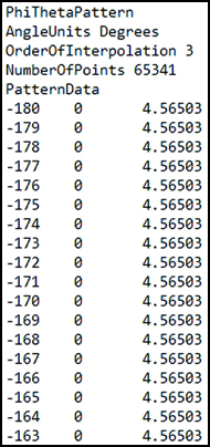
OmniIsolated Pattern File
Orienting the antenna
By default, the STK application places the antenna in a fixed 90-degree elevation on the satellite. You can reorient it and change the position of the antenna. Realistically, the antenna is not placed on the center of the model.
- Select the Basic - Orientation page.
- Set the following options:
- Set the following Position Offset values:
- Click to accept your changes and to keep the Properties Browser open.
| Option | Value |
|---|---|
| Azimuth | 270 deg |
| Elevation | 90 deg |
| Option | Value |
|---|---|
| X | -0.57 m |
| Y | 0.93 m |
| Z | 0.55 m |
Displaying contour graphics in the 2D Graphics window
The 2D Graphics Contours properties page for the antenna allows you to define the display of contour lines and antenna patterns.
- Select the 2D Graphics - Contours page.
- Select the Show Contour Graphics check box.
- Clear the Relative to Maximum check box.
- Set the following dB values in the Level Adding panel:
- Click .
- Click to accept your changes and to keep the Properties Browser open.
| Option | Value |
|---|---|
| Start | -10 |
| Stop | 11 |
| Step | 3 |
Displaying contour graphics in the 3D Graphics window
The 3D Graphics attributes page for the antenna allows you to control the 3D display of contour lines and antenna patterns.
- Select the 3D Graphics - Attributes page.
- Select the Show Lines check box in the Contour Graphics panel.
- Select the Show Volume check box in the Volume Graphics panel.
- Set the following options:
- Enter 180 deg in the Stop field in the Elevation panel.
- Open the Min Color drop-down list in the Gain Coloring panel.
- Select red.
- Open the Max Color drop-down list.
- Select blue.
- Click to accept your changes and to close the Properties Browser.
| Option | Value |
|---|---|
| Gain Scale (per dB) | 4 cm |
| Minimum Displayed Gain | -30 dB |
Renaming the Antenna
Rename the Antenna object to reflect that it is using the OmniIsolated antenna pattern.
- Right-click on Antenna1 () in the Object Browser.
- Select Rename in the shortcut menu.
- Rename Antenna1 () OmniIsolated.
Viewing the OmniIsolated antenna pattern in the 3D Graphics window
View the OmniIsolated antenna pattern in the 3D Graphics window.
- Bring the 3D Graphics window to the front.
- Right-click on LEO_Sat () in the Object Browser.
- Select Zoom To in the shortcut menu.
- Move around in the 3D Graphics window to understand the antenna pattern.
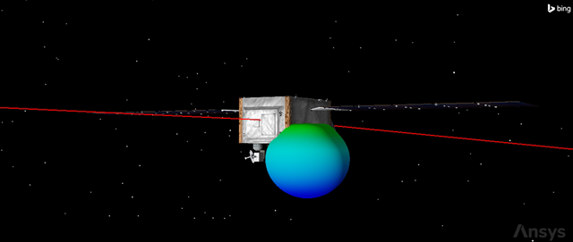
OmniIsolated antenna pattern
The antenna model is isolated from the model of the satellite. It does not take into account any aspect of the satellite that may affect the signal. The "perfect omni" antenna assumption may not be sufficient for RF link budget modeling.
Modifying the transmitter
You will analyze the behavior of this system to quantify it in detail. You can model a transmitter to house the antenna and compute the link budget. Transmitter objects can pull in configuration of antennas modeling in the scenario.
Using a Complex Transmitter model
Change the transmitter to use a Complex Transmitter model. A
- Open Transmitter's () Properties ().
- Select the Basic - Definition page in the Properties Browser.
- Click the Transmitter Model Component Selector ().
- Select Complex Transmitter Model () in the Transmitter Models list in the Select Component dialog box.
- Click to close the Select Component dialog box.
Changing the model specs
Update the model specs of the transmitter for your Complex Transmitter model.
- Select the Model Specs tab.
- Set the following options:
- Click to accept your changes and to keep the Properties Browser open.
| Option | Value |
|---|---|
| Frequency | 2.2 GHz |
| Power | 2 W |
Linking to an antenna object
You can select to embed an antenna model from the Component Browser or you can link to an antenna object.
- Select the Antenna tab.
- Open the Reference Type drop-down list.
- Select Link.
- Notice that Antenna/OmniIsolated is set as the Antenna Name.
- Click to accept your changes and to keep the Properties Browser open.
There are many default antenna gain patterns available in the STK application. Instead of these, you can load an external antenna pattern that is relevant to the mission.
Refreshing the Link Budget report
Refresh your Link Budget report to examine the effects of your changes.
- Bring the Link Budget report to the front.
- Click Refresh (F5) (
 ) in the report's toolbar.
Notice the increased variation in the BER with this updated model. Rather than a constant value, see how the BER varies throughout the satellite's passage. However, this is still an idealized mission model; realistically, the behavior of the antenna changes depending on how it is placed on the body of the satellite. You will analyze that behavior next.
Modeling the OmniInstalled antenna
The relationship between the vehicle and its payload can dramatically alter antenna performance and impact the associated system. This is important to take into account in the mission model. To account for the satellite model behavior, you must use the OmniInstalled antenna pattern file. This file models the antenna's behavior; assuming the antenna was installed at a specific location on the body of the vehicle, it would take into account the interference from that location.
The OmniInstalled file was created using the

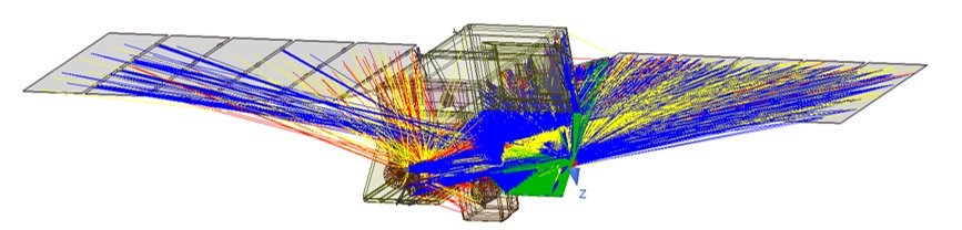
The figures above demonstrate the results from HFSS SBR+ using Shooting and Bouncing Rays analysis.
However, the antenna behavior data could come from a multitude of sources: you can create your own data using the STK software, load external models, and load results from system tests.
Reusing the OmniIsolated antenna
You can reuse objects in the STK software.
- Right-click on OmniIsolated () in the Object Browser.
- Select Copy (
 ) in the shortcut menu.
 - Right-click on LEO_Sat () in the Object Browser.
- Select Paste (
 ) in the shortcut menu.
 - Rename OmniIsolated1 () OmniInstalled.
- Clear the OmniIsolated () check box in the Object Browser.
Updating OmniInstalled's properties
Update the OmniInstalled antenna to use the OmniInstalled antenna pattern.
- Open OmniInstalled's () Properties ().
- Select the Basic - Definition page in the Properties Browser.
- Click the External Filename ellipsis ().
- Browse to the location of your pattern file (e.g. C:\Users\<username>\Documents\STK_ODTK 13\DME_Session3_Starter_Comms\DME_CommAnalysis_Part3) in the Select File dialog box.
- Select SatCom_Omni_2p2G_Installed.pattern.
- Click .
- Click to accept your changes and to close the Properties Browser.
If you open the pattern file in a text editor, you will notice that the values change throughout the file.

OmniINstalled Pattern file
Viewing the OmniInstalled antenna pattern in the 3D Graphics window
See the dramatic difference between the two antenna models.
- Bring the 3D Graphics window to the front.
- Right-click on LEO_Sat () in the Object Browser.
- Select Zoom To in the shortcut menu.
- Move around in the 3D Graphics window to understand the new antenna pattern.
It is also important to understand the effect the interaction of the antenna and satellite can have on the signal. This is visualized with the contours on the surface of the Earth. The effects can also be measured in the data.
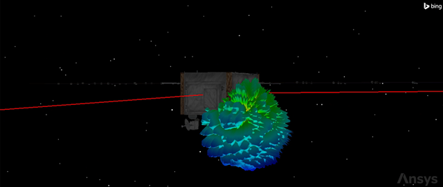
OmniInstalled antenna pattern
Switching to the OmniInstalled antenna
Set your transmitter to use the OmniInstalled antenna.
- Open Transmitter's () Properties ().
- Select the Antenna tab in the Basic - Definition page of the Properties Browser.
- Select the Model Specs sub tab.
- Open the Antenna drop-down list.
- Select Antenna/OmniInstalled.
- Click to accept your changes and to close the Properties Browser.
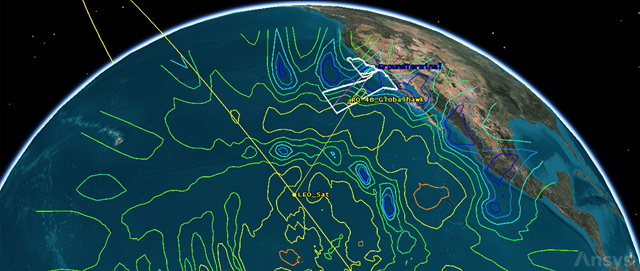
Viewing the OmniInstalled antenna contours in the 3D Graphics window
View the changes to the antenna contours in the 3D Graphics window.
- Bring the 3D Graphics window to the front.
- Right-click on LEO_Sat () in the Object Browser.
- Select Zoom To in the shortcut menu.
- Move around in the 3D Graphics window to view the contours on the Earth.
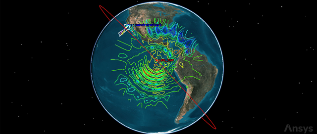
OmniInstalled Antenna Contours
Over time, the antenna pattern passes over the Ground Terminal. You can assess it in more detail with a bit error rate graph.
Refreshing the Link Budget report
Examine the changes to your Link Budget report.
- Bring the Link Budget report to the front.
- Click Refresh (F5) () in the report's toolbar.
Notice the variations in the bit error rate. To understand how this antenna model affects the data, you can generate a BER graph.
Generating a BER graph
A BER graph plots the bit error rate over time, during each access interval.
- Right-click on OmniInstalled () in the Object Browser.
- Select Report & Graph Manager... (
 ) in the shortcut menu to open the Report & Graph Manager.
 - Select Access in Object Type drop-down list.
- Select Satellite-LEO_Sat-Transmitter-Transmitter-To-Facility-GroundTerminal-Receiver-Receiver (
 ) in the Object Type list.
 - Expand () Installed Styles (
 ) in the Styles panel if needed.
 - Select the Bit_Error_Rate (
 ) graph.
 - Click .
- Enter 1 sec in the Step field.
- Refresh (F5) () in the report's toolbar.
- Hold down your left mouse button and draw a bounding outline around one of the peaks. This zooms into the selected region to show the data values.
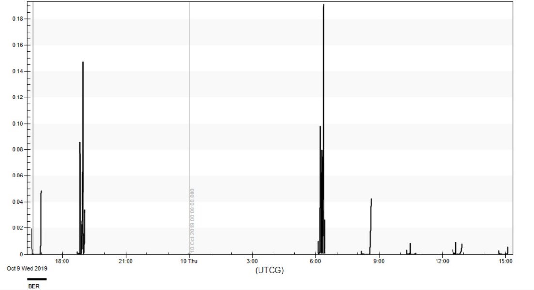
bit error rate graph throughout the scenario
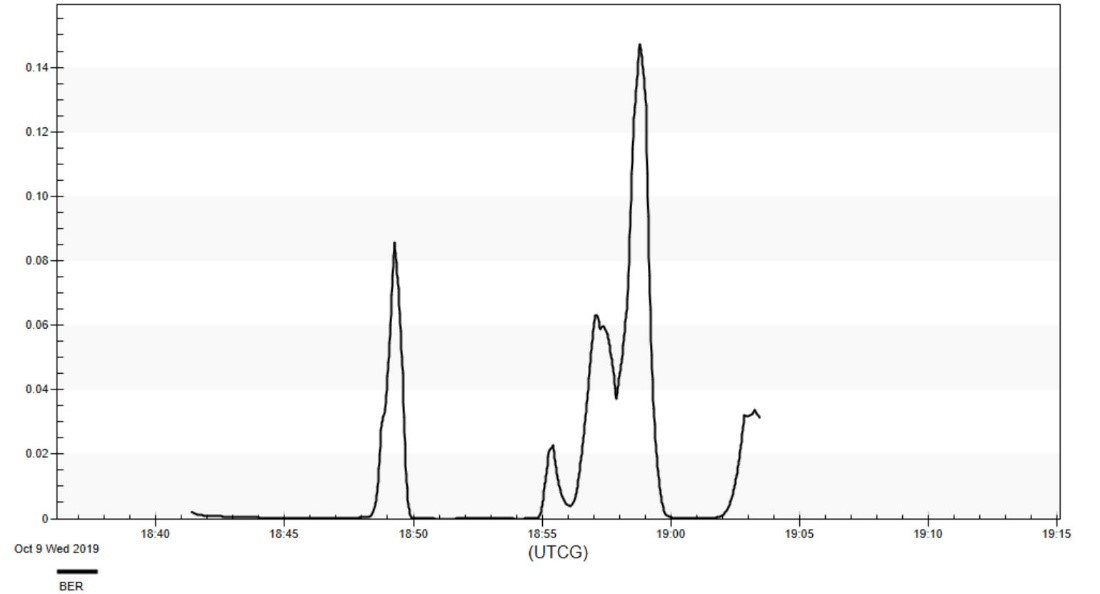
zoomed-in bit error rate graph
Obtaining situational awareness with the 3D Graphics window
You can jump to a time in your graph and obtain situational awareness in the 3D Graphics window.
- Right-click on the sharp peak in the graph.
- Select Set Animation Time in the shortcut menu.
- Bring the 3D Graphics window to the front.
- Zoom to LEO_Sat ().
- Move around in the 3D Graphics window to note the dip in the antenna pattern as it passes over the GroundTerminal ().
- Clear the OmniInstalled () check box in the Object Browser.
3D Graphics View: Antenna Pattern over Ground Terminal
It is important to consider how you would not have known when bit error rates increased had you not used a custom external antenna model and generated the BER graph.
Designing a satellite collection
From your preliminary analysis, you found that six satellites in six orbital planes are required to maintain worldwide coverage, for a total of 36 satellites. You can model this constellation with a Satellite Collection object. A
Inserting a Satellite Collection object
Insert a new Walker satellite collection using the
- Insert a Satellite Collection (
 ) object using the Walker Tool () method.
 - Click in the Walker Tool dialog box.
- Select LEO_Sat () in the Select Object dialog box.
- Click to close the Select Object dialog box.
- Set the following options:
- Enter LEO_Sats in the Name field in the Container Options panel.
- Click .
- Click to close the Walker Tool dialog box.
| Option | Value |
|---|---|
| Number of Sats per Plane | 6 |
| Number of Planes | 6 |
Displaying the satellite collection labels
You can control the graphical display of a satellite collection. You want to display the satellites' names next to their markers for each satellite in the subset for situational awareness.
- Open LEO_Sats' () Properties ().
- Select the Graphics - Attributes page in the Properties Browser.
- Select the AllSatellites Label check box.
- Click to accept your change and to close the Properties Browser.
Viewing the satellite collection
View the labeled satellites in the 3D Graphics window.
- Bring the 3D Graphics window to the front.
- Move around in the 3D Graphics window to the constellation of satellites.

Walker constellation
Creating a Chain object
You built a global constellation to provide as much coverage as possible to track the hypersonic vehicle. However, not all of these satellites are overhead during the time of the flight. You only care about a subset of the satellites, not all 36 satellites. Use a
Inserting a new Chain object
Start by inserting a new Chain object.
- Insert a Chain (
 ) object using the Insert Default () method.
 - Rename Chain1 () LEO_to_Ground.
Defining the start and end objects
Start by choosing the start object and end object in your chain.
- Open LEO_to_Ground's () Properties ().
- Select the Basic - Definition page in the Properties Browser.
- Click the Start Object ellipsis ().
- Select AllSatellites (
 ) in the Select Object dialog box.
 - Click to close the Select Object dialog box.
- Click the End Object ellipsis ().
- Select GroundTerminal () in the Select Object dialog box.
- Click to close the Select Object dialog box.
Creating the Chain object's connections
After you choose the start and end objects in your chain, you need to build the chain's connections. It doesn't matter in which order you place the connections in the Connections list. What matters is the From Object must be able to access the To Object.
- Click in the Connections panel.
- Click the From Object ellipsis ().
- Select AllSatellites () in the Select Object dialog box.
- Click to close the Select Object dialog box.
- Click the To Object ellipsis ().
- Select GroundTerminal () in the Select Object dialog box.
- Click to close the Select Object dialog box.
- Click to accept your changes and to close the Properties Browser.
You can calculate this analysis with the transmitters and receivers. When you use an entry of a satellite collection in your analysis, that entry will inherit the properties of a reference object. By default, the reference object is simply the default satellite object. However, if you choose a default subset reference object, the STK software will associate the entries with that specific satellite in the scenario. Using a specified satellite provides a way to customize settings (attitude, access constraints, etc.) when you use the satellite collection member in an analysis. Moreover, when the reference object contains child objects (sensors, transmitters, receivers, etc.), The STK software also associates these children with the satellite entry.
Generating an Individual Strand Access graph
An Individual Strand Access Individual Strand Access graph displays the time intervals for each strand in a chain that completes the chain. Each strand's intervals are graphed on a separate line.
- Right-click on LEO_to_Ground () in the Object Browser.
- Select Report & Graph Manager... () in the shortcut menu.
- Select the Individual Strand Access () graph in the Installed Styles list.
- Click .
- Close the Individual Strand Access graph when done viewing the data.
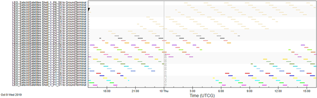
individual strand access graph
Defining custom availability intervals
Throughout the period of analysis, you can see all the links between your satellites and the ground terminal. However, you care about how these systems communicate during the period of the X-43's test flight. You can use Availability Intervals to figure out which satellites are relevant during the flight.
- Return to the Report & Graph Manager.
- Select the Specify Time Properties option in the Time Properties panel.
- Open the Select Type drop-down list.
- Select Custom Interval List.
- Click the ellipsis ().
- Select HXRV_X43 (
 ) in the object list in the Select Interval List dialog box.
 - Select AvailabilityIntervals (
 ) from the Interval Lists for HXRV_X43 list.
 - Click to close the Select Interval List dialog box.
- Select the Individual Strand Access () graph in the Installed Styles list.
- Click .
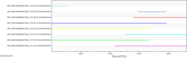
Modified Individual Strand Access
Now you are just looking at the eight satellites overhead during the time of the flight. Through each stage of the analysis, you needed to reevaluate the outcomes of the mission. Through modifications of the antenna and examining the link budget, you can see the effects through each iteration. This falls directly in line with the DME workflow. Within one system (the STK software), changing the necessary systems (transmitters) maintain the required mission metrics (Link Budget - BER).
Saving your work
You can clean up and finish your scenario.
- Close any open graphs, properties, and tools.
- Save (
 ) your work.
Summary
The purpose of this series and this lesson is to evaluate how all the components of the mission work together. In previous sessions, you built detailed models, and in this scenario you determined which satellites in a constellation of satellites can talk to a ground terminal during the flight of the X-43 HXRV.
DME: Events and Time Components
The