STK Premium (Space) or STK Enterprise
You can obtain the necessary licenses for this tutorial by contacting AGI Support at support@agi.com or 1-800-924-7244.
This lesson requires version 12.7 of the STK software or newer to complete.
Required product install: The Ansys ModelCenter® model-based systems engineering software and the STK Plugin for ModelCenter are required to complete this tutorial.
ModelCenter installation prerequisites: The ModelCenter software requires the installation of a 64-bit version of Java, a 64-bit implementation of Python 3.x, and the installation of the thrift and six Python packages. See the ModelCenter Installation Prerequisites for more information.
This tutorial was written using version 2026 R1 of the Ansys ModelCenter® model-based systems engineering software.
The results of the tutorial may vary depending on the user settings and data enabled (online operations, terrain server, dynamic Earth data, etc.). It is acceptable to have different results.
Capabilities covered
This lesson covers the following capabilities of the Ansys Systems Tool Kit® (STK®) digital mission engineering software:
- STK Pro
- Coverage
- STK Analyzer
- STK Analyzer Optimization
Problem statement
Across the industry, the digital engineering process is becoming more complex. Systems of systems are being changed and updated in different stages of the mission life cycle. In this series, you will address these challenges by creating a fully connected digital thread with a common mission environment at the core. You will address this topic in stages: satellite constellations, hypersonic flight, EOIR sensors, communications links, and triggering events and systems. The vision is to integrate the mission environment and operational objectives into the digital thread early and throughout the entire product life cycle. Through digital mission engineering, you are now capable of quickly evaluating the overall mission impact of the smallest change to any component. This session will focus on the concept development phases using the Ansys ModelCenter® model-based systems engineering software. You want to design, test, and optimize a new satellite constellation for persistent stereo coverage of hypersonic vehicles across the world.
Solution
Use the STK software's Coverage capability and the Analyzer capability, which is available with the Ansys ModelCenter® model-based systems engineering software, to conduct trade studies on the satellite constellation's geometry and optimize it based on mission and system requirements. The goal in this exercise is to understand how to maximize the level of global coverage with a network of satellites. The main components you will analyze are the revisit time, which can be considered the gap time, and the number of assets that have visibility to a point on the Earth's surface at a given time. Using the STK Analyzer Optimization capability and the ModelCenter software's trade study capabilities, you can vary parameters of your system to find an ideal configuration.
What you will learn
Upon completion of this tutorial, you will be able to:
- Build a constellation of satellites using the Satellite Collection object
- Design a Coverage analysis
- Utilize relevant Figure of Merit quality metrics
- Become familiar with the ModelCenter software's workflow
- View an external trade study file
- Understand satellite constellation design configurations
Creating a new scenario
First, you must create a new scenario and then build from there.
- Launch the STK application (
 ).
). - Click
 Create a Scenario in the Welcome to STK dialog box.
 - Enter the following in the STK: New Scenario Wizard:
- Click when you finish.
- Click Save (
 ) when the scenario loads. The STK application creates a folder with the same name as your Scenario for you.
 - Verify the scenario name and location in the Save As dialog box.
- Click .
| Option | Value |
|---|---|
| Name | ImagingConstellation |
| Start | 13 Feb 2025 16:00:00.000 UTCG |
| Stop | + 1 day |
Save (![]() ) often during this lesson!
) often during this lesson!
Downloading a precomputed trade study
This tutorial uses a precomputed trade study. Download it following the steps below.
- Download the zipped folder here: https://support.agi.com/download/?type=training&dir=sdf/help&file=DME_Part1_MC_TradeStudy.zip
If you are not already logged in, you will be prompted to log in to agi.com to download the file. If you do not have an agi.com account, you will need to create one. The user approval process can take up to three (3) business days. Please contact support@agi.com if you need access sooner.
- Navigate to the downloaded folder in Windows File Explorer.
- Right-click on DME_Part1_MC_TradeStudy.zip.
- Select Extract All... in the shortcut menu.
- Set the Files will be extracted to this folder: path to your scenario folder (for example, C:\Users\<username>\Documents\STK_ODTK 13\ImagingConstellation).
- Click .
- Navigate to your scenario folder.
- The DME_OptStudy3.tstudy file will be in your scenario folder.
Creating a Walker-type Satellite Collection
A Satellite Collection object models a group of satellites as a single object in the Object Browser. The associated satellites do not appear in the Object Browser, but are available for analysis purposes within other computational tools such as the STK software's Coverage capability, CommSystem objects, the Deck Access tool, and the Advanced CAT tool.
Inserting a Satellite Collection object
Start by inserting a Satellite Collection object into your scenario.
- Bring the Insert STK Objects tool (
 ) to the front.
 - Select SatelliteCollection (
 ) in the Select An Object To Be Inserted list.
 - Select Insert Default () in the Select A Method list.
- Click .
- Right-click on SatelliteCollection1 () in the Object Browser.
- Select Rename in the shortcut menu.
- Rename SatelliteCollection1 () Walker_Collection.
Setting the Walker type subset
The default
- Right-click on Walker_Collection () in the Object Browser.
- Select Properties (
 ) in the shortcut menu.
 - Select the Basic - Definition page when the Properties Browser opens.
- Select the Shells - Name - 1 row in the Walker Properties panel.
- Click Edit selected shell (
 ) in the Shells toolbar.
 - Enter Walker Group in the Shell Name field when the Edit Shell dialog box opens.
- Set the following options in the order shown in Shell Properties panel:
- Set the following orbital parameters in the Plane 1 : Slot 1 panel:
- Click to apply your changes and to close the Edit Shell dialog box.
- Click to accept your changes and to keep the Properties Browser open.
You can see that Walker is selected as the default Type.
| Option | Value |
|---|---|
| Inter Plane Phase Increment | 0 |
| Planes | 1 |
| Satellites in Planes (Slots) | 1 |
| Option | Value |
|---|---|
| Semi-Major Axis (a) | 6880 km |
| Inclination (i) | 50 deg |
Setting the subset marker size
You can control the graphical display of a satellite collection. The Satellite Collection
- Select the Graphics - Attributes page.
- Double-click in the AllSatellites - Marker Size cell.
- Enter 10 as the Marker Size value.
- Click to accept your changes and to close the Properties Browser.
Using a Coverage Definition object
You are now ready to model a coverage analysis over the Earth using a
Inserting a Coverage Definition object
Start by inserting a Coverage Definition object using the Define Properties method.
- Bring the Insert STK Objects tool () to the front.
- Select Coverage Definition (
 ) in the Select An Object To Be Inserted list.
 - Select the Define Properties () method in the Select A Method list.
- Click .
Changing the grid area of interest and point granularity
Coverage analyses are based on the accessibility of assets (objects that provide coverage) and geographical areas. The combination of the geographical area, the regions within that area, and the points within each region is called the
Use the Grid properties to define the location of your coverage grid to fall between specified minimum and maximum latitude bounds, with a point granularity that balances for accuracy and computation time.
- Select the Basic - Grid page when the Properties Browser opens.
- Enter 60 deg in the Max. Latitude field in the Grid Area of Interest panel.
- Enter 10 deg in the Lat/Lon field in the Point Granularity panel located in the Grid Definition panel.
- Click to accept your changes and to keep the Properties Browser open.
Specifying the coverage assets
- Select the Basic - Assets page.
- Expand (
 ) Walker_Collection () in the Assets list.
 - Select the AllSatellites (
 ) Satellite Collection subset.
 - Click .
- Click to accept your changes and to keep the Properties Browser open.
Clearing Automatically Recompute Accesses
The STK application automatically recomputes accesses every time you update an asset on which the coverage definition depends, such as your Satellite Collection object. If you want to control when the STK software computes coverage, you need to turn this option off in the Coverage Definition object's
- Select the Basic - Advanced page.
- Clear the Automatically Recompute Accesses check box.
- Click to accept your changes and to close the Properties Browser.
- Rename CoverageDefinition1 () CoverageDefinition.
Using the Compute Accesses tool
The ultimate goal of coverage is to analyze accesses to an area by using assigned assets and applying necessary limitations upon those accesses. Compute coverage with the Compute Accesses tool.
- Right-click on CoverageDefinition () in the Object Browser.
- Select CoverageDefinition in the shortcut menu.
- Select Compute Accesses in the CoverageDefinition submenu.
Generating a Percent Coverage graph
Now that you have set up and computed the coverage analysis, you can examine the quality of the coverage. But before you do that, take a quick look at the quality of the system you set up. One way to do that is to generate a
- Select the Analysis menu.
- Select Report & Graph Manager... (
 ).
). - Open the Object Type drop-down list when the Report & Graph Manager opens.
- Select CoverageDefinition.
- Select CoverageDefinition () in the Object Type list.
- Select the Percent Coverage (
 ) graph in the Installed Styles (
 ) folder inside the Styles panel.
 - Click .
- Close the Percent Coverage graph and the Report & Graph Manager.

Percent Coverage graph
Take a look at how the current coverage stays low throughout the analysis period, but how the accumulated coverage increases over time. This gives you an idea of how well a single satellite can cover the region. You can understand this further with a Figure of Merit object.
Designing the coverage definition Figures of Merit
You set up the problem using a Coverage Definition object. The STK software enables you to specify the method by which the quality of coverage is measured using a Figure Of Merit object. You can attach FOM objects to a Coverage Definition object; they provide the means for evaluating the quality of coverage provided by Coverage Definition's assigned objects (or assets).
In this study, you will focus on two parameters: the Number of Assets (N Asset Coverage) and the Revisit Time. The mission requirements state you must have at least two assets covering every grid point at all times.
Inserting an N Asset Figure of Merit object
An
You can specify that the FOM compute the minimum value from the set of all grid points to make sure all grid points are at or above that threshold.
- Insert a Figure of Merit (
 ) object using the Define Properties () method.
 - Select CoverageDefinition () in the Object Tree when the Select Object dialog box opens.
- Click to confirm your selection and to close the Select Object dialog box.
Setting the N Asset coverage definition
You want to measure if at least two satellites simultaneously cover every single point in the coverage analysis.
- Select the Basic - Definition page when the Properties Browser opens.
- Open the Type drop-down list in the Definition panel.
- Select N Asset Coverage.
- Open the Compute drop-down list.
- Select Minimum.
Using Minimum calculates the minimum number of assets available over the entire coverage interval.
Selecting the N Asset FOM satisfaction criterion
You can restrict the FOM's behavior so that the STK application only applies the graphical properties of the FOM when a chosen
- Select the Enable check box in the Satisfaction panel.
- Open the Satisfied if drop-down list.
- Select At Least.
- Enter 2 in the Threshold field.
- Click to accept your changes and to close the Properties Browser.
- Rename FigureofMerit1 () NAsset.
Satisfaction is achieved when the FOM value is greater than or equal to the Threshold.
Inserting the revisit time Figure of Merit object
Now that the coverage has a threshold of at least two satellites per grid point, you can set up a new figure of merit for the revisit or gap time.
- Insert a Figure of Merit () object using the Define Properties () method.
- Select CoverageDefinition () in the Object Tree when the Select Object dialog box opens.
- Click to confirm your selection and to close the Select Object dialog box.
Defining the revisit time coverage definition
- Select the Basic - Definition page when the Properties Browser opens.
- Open the Type drop-down list in the Definition panel.
- Select Revisit Time.
- Enter 2 in the Min # Assets field.
- Keep the Compute and End Gaps options set as their default selections.
Min # Assets specifies the minimum number of simultaneous assets that are required for coverage.
Compute - Maximum specifies that the computed value is the duration of the longest gap in coverage over the entire coverage interval. Setting the End Gaps to Include has gaps at the ends of the analysis interval included in your revisit time computations.
Selecting the revisit time FOM satisfaction criteria
You will use the At Most Satisfaction Criteria. Using At Most, the FOM value is less than or equal to the Threshold value.
- Select the Enable check box in the Satisfaction panel.
- Open the Satisfied if drop-down list.
- Select At Most.
- Leave the default Threshold value of 0 sec.
- Click to accept your changes and to close the Properties Browser.
- Rename FigureofMerit2 () RevisitTime.
At this point, you might be wondering why you're setting up both FOMs to use a minimum of two satellites when you currently have one satellite in your collection. When you use the ModelCenter software, you will set it up so that there are six orbital planes with six satellites per plane.
Closing out of the STK application
With your baseline scenario configured, save your scenario and close out of the STK application in preparation for the next step.
- Save () your scenario.
- Close any open reports, the Report & Graph Manager, and any open tools.
- Close the STK application.
Creating a new ModelCenter project
The
- Open the ModelCenter (
 ) application.
 - Click in the Welcome to ModelCenter dialog box.
- Click when the What type of model would you like to create? dialog box opens.
- Navigate to your scenario folder (for example, C:\Users\<username>\Documents\STK_ODTK 13\ImagingConstellation.
- Enter ImagingConstellation in the File name field.
- Ensure the Save as type is set to the ModelCenter Model (Zip) (*.pxcz).
- Click .
Using the STK Plugin for ModelCenter
The
- Select favorites (
 ) in the Server Browser at the bottom of the window.
 - Click and drag the STK component (
 ) into the dashed circle underneath "Drop items here to build the model" in the workflow's Analysis View.
 - Select ImagingConstellation.sc when the Open STK Scenario file dialog box opens.
- Click .
- After a few moments, the STK Analyzer window will open.
The ImagingConstellation scenario file will open in the STK application in the background.
Setting up your analysis with Analyzer
You are now ready to dive into some trade study analysis using the ModelCenter software. You can build a simple example and then load the results into a more complex study. The goal is to become familiar with the Analyzer workflow in the ModelCenter application, as well as loading results of previously run analyses.
Selecting the input variables
Use the STK Analyzer window to configure the input and output variables available for further analysis with the
- Select Walker_Collection () in the STK Variables tree.
- Select the Walker (
 ) property in the STK Property Variables tree.
 - Move (
 ) Walker () to the Analyzer Variables list.
Note that your Walker constellation's orbital parameters, including the Argument of Periapsis, Eccentricity, Inclination, Planes, RAAN, and more have all be added as Inputs in the Analyzer Variables list.
Defining the output variables
Now that the input variables are defined, you can add the output variables. The output variables are the variables you'd like to solve for. You want to solve for Minimum N Asset Overall and Maximum Revisit Time Overall. The same data providers that are available in the Report & Graph Manager in the STK application are available in the Data Provider Variables tree.
- Expand (
 ) CoverageDefinition () in the STK Variables tree.
 - Select NAsset ().
- Expand () the Overall Value (
 ) data provider in the Data Provider Variables tree.
 - Select the Minimum (
 ) data provider element.
 - Move () Minimum () to the Analyzer Variables list.
- Select RevisitTime () in the STK Variables tree.
- Expand () the Overall Value () data provider.
- Select the Maximum () data provider element.
- Move () Maximum () to the Analyzer Variables list.
- Click to accept your changes and to close the STK Analyzer window.
Note that both FOM values have been added as Outputs in the Analyzer Variables list.
This will also close the STK application, which had been running in the background.
Using the Parametric Study tool
The Parametric Study tool runs a model through a sweep of values for some input variable. The resulting data can be plotted to view trends.
Specifying the variables
To perform a Parametric Study, one design variable and one or more responses must be specified. For the design variable, a starting value, an ending value, and the number of steps must be specified.
- Expand () all the elements in the Component Tree.
- Click Parametric Study (
 ) in the Standard toolbar.
 - Click and drag SemiMajorAxis (
 ) from the Component Tree to the Design Variable field when the Parametric Study tool opens.
 - Set the following Design Variable values:
- Click and drag NAsset - Overall_Value - Minimum (
 ) and RevisitTime - Overall_Value - Maximum () from the Component Tree to the Responses list:
| Option | Value |
|---|---|
| starting value | 6880 |
| ending value | 7680 |
| step size | 100 |
Note the number of samples is automatically set to 9. These settings will vary the semi-major axis in 100-kilometer increments. It will take a total of nine runs to complete the trade study.
Defining the Walker variables
Define the walker parameters within the parametric study.
- Locate the Walker - Shell_Walker_Group list, located in the Component Tree. To the right of each variable is a value that you can click to change the value.
- Set the following options for Walker_Constellation:
| Name | Value |
|---|---|
| Planes | 6 |
| SatellitesInPlanes | 6 |
Running the parametric trade study
This parametric trade study will take a few minutes to run.
- Click .
- Close the 2D Scatter Plot that opened when the trade study finished running.
Clicking will open the Data Explorer, which is a tool used by Trade Study tools to display data collected from a Model. While data are being collected, the Data Explorer displays a progress meter, a halt button, and the data. In each of the runs, you should see the revisit time (gaps) decrease as the semi-major axis increases. Eventually, it goes to zero. The average increases to two for the number of assets. The minimum number of assets eventually reaches two.
Generating a 3D Scatter Plot
There are a few ways to view the data. One interactive way to view the data is with a 3D Scatter Plot. A 3D Scatter Plot displays an x-y plot of variables in the model.
- Bring the Table page to the front when all runs finish.
- Click Add View (
 ) on the Table page toolbar.
 - Select 3D Scatter Plot (
 ) in the drop-down menu.
Modifying the 3D Scatter Plot
Use the Plot Options menu to change which variable is displayed on which axis.
- Click Dimensions in the Plot Options menu when the 3D Scatter Plot opens.
- Set the following options:
- Click anywhere on the graph to close the Plot Options menu.
| Option | Value |
|---|---|
| x | Maximum |
| y | Minimum |
| z | SemiMajorAxis |
Reviewing the 3D Scatter Plot
Examine the 3D Scatter Plot.
- Hover over any design point to get information about that run.
- Close the 3D Scatter Plot and the Table page when you are finished.
- Click when prompted to close your trade study without saving.
- Close the Parametric Study tool.
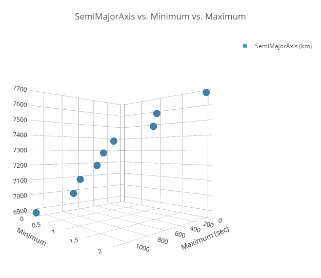
ModelCenter 3D Scatter plot
Note the semi-major axis of the last run (7,680 km). This gives you the requirements you are looking for: 2 assets with a 0-second revisit time.
Saving the results of your parametric study
All of the criteria meet in the final run, whose semi-major axis is 7,680 km; however, remember that the semi-major axis values are raised in 100-kilometer increments. There is likely a minimum semi-major axis that enables you to achieve your goals sooner. If you consider cost, which might be tied to a higher orbit, you can find a lower semi-major axis that also reduces cost.
Push the results of a single run to the STK application and examine the scenario.
- Enter 7680 as the Value for the SemiMajorAxis input variable in the Component Tree.
- Click Save (
 ) to save your ModelCenter workflow.
 - Keep the ModelCenter application open.
You do not need to enter units.
Updating your STK scenario
Update your Walker Collection with the data from the last run in your trade study.
- Reopen the STK application ().
- Reopen your ImagingConstellation scenario.
- Open Walker_Collections' () Properties ().
- Select the Walker Group row in the Walker Properties panel.
- Click Edit selected shell () in the Shells toolbar.
- Set the following options in the Shell Properties panel when the Edit Shell dialog box opens:
- Set Semi-Major Axis (a) to 7680 km.
- Click to confirm your changes and to close the Edit Shell dialog box.
- Click to confirm your changes and to close the Properties Browser.
| Name | Value |
|---|---|
| Planes | 6 |
| SatellitesInPlanes | 6 |
Recomputing the accesses
With your Walker Satellite Collection updated, recompute the accesses.
- Right-click on CoverageDefinition () in the Object Browser.
- Select CoverageDefinition in the shortcut menu.
- Select Compute Accesses in the CoverageDefinition submenu.
Examining the data
Now that you have a result loaded in, look at some of the reports and graphs in the STK application that can shed some light on the scenario.
Generating a Percent Satisfied report
A
- Right-click on NAsset () in the Object Browser.
- Select Report & Graph Manager... () in the shortcut menu.
- Select the Percent Satisfied (
 ) report in the Installed Styles () folder when the Report & Graph Manager opens.
 - Click .
- Scroll to the bottom of the report and look at the % Satisfied column.
- Close the Percent Satisfied report.
You should have 100% satisfaction, which means you have a minimum of two satellites with access to every point in the coverage grid. The Percent Satisfied report confirms that information.
Generating a Grids Stats Over Time report
A
- Select the Grids Stats Over Time () report in the Installed Styles () folder.
- Click .
- Scroll through the report.
- Continue to test configurations using parametric scans, carpet studies, and design of experiments.
- Optimize the scenario to find the optimal semi-major axis.
You can see that you meet the minimum, but you have a few locations that have up to five or six satellites with access (depending on the analysis period). This creates a lot of redundancies, so you can start thinking of optimizing the setup.
You have two options at this point:
You may also consider if you need to change other factors with the study, such as number of satellites or planes.
Closing out of the STK application
With your scenario reconfigured, save your scenario and close out of the STK application in preparation for the next step.
- Close any open reports and the Report & Graph Manager when finished.
- Save () your scenario.
- Close any open reports, the Report & Graph Manager, and any open tools.
- Close the STK application.
Loading a precomputed optimization trade study
The study you will load in was run for approximately an hour using the Satellite Collection object. Older versions of the STK software required the use of the Walker Tool and individual Satellite objects, which took upwards of 10 hours to analyze. The goal is to minimize the semi-major axis and the total number of satellites. At the same time, you want to minimize the revisit time (no gaps) and have two satellites maintain access with a point on the ground.
Opening the precomputed trade study
Load in the data from the precomputed trade study and examine it.
- Return to the ModelCenter application.
- Click Open (
 ) on the Standard Toolbar.
 - Browse to the location of the precomputed trade study you extracted earlier (for example, C:\Users\<username>\Documents\STK_ODTK 13\ImagingConstellation).
- Select DME_OptStudy3.tstudy (
 ).
). - Click .
This opens the Optimization tool, a 3D Scatter Plot, and the trade study's Table page.
Understanding the results
View the results in the precomputed trade study's 3D Scatter Plot.
- Bring the 3D Scatter Plot window to the front.
- Examine the 3D Scatter Plot.
- Hover over any design point in the graph to see more information about a run.
- Select the feasible design point with the lowest semi-major axis.
- Bring the Data Explorer window to the front.
- Examine the runs on the Table page.
- Scroll to run 278.
You can see the configurations that met the criteria in blue and those that didn't in gray.
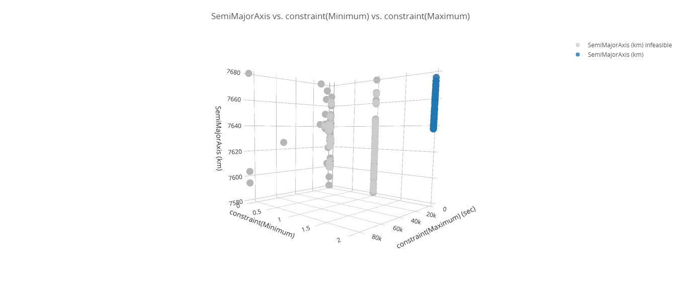
ModelCenter Optimization tool 3D Scatter plot
This is the lowest semi-major axis that satisfies all of your criteria, which, for this trade study, was design point 278, with a semi-major axis of 7637.6 km.
You can scroll to see all the runs that were conducted and each result. You also have the option to export the data into Excel or another tool for post-processing.
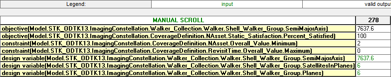
Table View showing best run
This is the run that best met all of the criteria of the trade study.
If you want to run the trade study yourself, proceed to the Performing an Optimization Study section. Otherwise, skip to Saving your model section.
Performing an Optimization Study
Looking at the data, there is a clear point that meets all the conditions for the study. Use the STK Analyzer Optimization capability, by means of the ModelCenter software's Optimization tool, to get an idea of the workflow. The Optimization tool is a collection of optimization algorithms that you can use within the ModelCenter application. A common graphical user interface (GUI) is provided to define optimization problems. An algorithm selection wizard is also provided to make it easy to choose algorithms that will work best for the problem at hand.
This is an additional section for users who would like to set up an optimization themselves.
Closing out your trade study
Close out the precomputed trade study.
- Close the 3D Scatter Plot.
- Close the Data Explorer window.
- Close the Optimization tool.
Adding an additional output variable
You want to make sure you maintain 100% coverage satisfaction across your area of interest with your optimized solution. Add the NAsset Figure of Merit's Percent Satisfied output variable to use as an objective in your optimization study.
- Right-click on the STK_ODTK13 component in the Analysis View.
- Select Show Component's GUI (
 ) in the shortcut menu.
 - Expand () CoverageDefinition () in the STK Variables tree when the STK Analyzer window opens.
- Select NAsset ().
- Expand () the Static Satisfaction () data provider.
- Select the Percent Satisfied () data provider element.
- Move () Percent Satisfied () to the Analyzer Variables list.
- Click to accept your changes and to close the STK Analyzer window.
Defining the optimization objective
To perform an Optimization Study, an objective function and a least one design variable must be specified. The objective functions can be specific variables or equations composed of multiple output variables. For each objective, you must specify whether you want to minimize or maximize the objective or find a design where the objective has as specific value. Your current objective is to minimize the semi-major axis while meeting the coverage criteria.
- Click Optimization Tool (
 ) on the Standard Toolbar.
 - Expand () all components in the Component Tree.
- Click and drag SemiMajorAxis () from the Component Tree to the Objective field when the Optimization tool opens.
- Ensure the Goal is set to minimize.
- Click and drag Percent_Satisfied () from the Component Tree to the Objective field.
- Open the Goal drop-down menu (
 ) for Percent_Satisfied.
 - Select maximize.
You want to ensure that your solution maximizes the coverage at 100% to conclusively rule out any combinations that provide less than full coverage.
Defining the constraints
Constraints restrict particular variables to a region or value, that is, a bound specified in the list of constraints prevents a design point from being found that causes that output variable to occur outside the specified region. For this optimization, you want to minimize the number of satellites that will provide coverage without any gaps.
- Click and drag NAsset - Overall_Value - Minimum () from the Component Tree to the Constraint field.
- Set the Lower Bound to 2.
- Leave the Upper Bound blank.
- Click and drag Revisit Time - Overall_Value - Maximum () from the Component Tree to the Constraint field.
- Set the Lower and Upper Bounds to 0.
Each constraint must have either an upper or lower bound, but can also have both. Constraints can also be equations composed of multiple variables.
Defining the SemiMajorAxis design variable
The design variables are the variables that the optimizer will modify to meet the objective. You must enter the bounds between which the optimizer is allowed to set the design variables. For continuous variables, like the semi-major axis, these bounds are required.
- Click and drag SemiMajorAxis () from the Component Tree to the Design Variable field.
- Set the following Lower and Upper bounds:
| Option | Value |
|---|---|
| Lower Bound | 7580 |
| Upper Bound | 7680 |
Defining the number of satellites per plane
Optimize for the number of satellites per plane. Both the start and end values must be specified for the number of satellites, which is defined by an integer value. The start and end values are used to create the enumeration for the integer; all integer values between the start and end values are used.
- Click and drag SatellitesInPlanes () from the Component Tree to Design Variable field.
- Set the following options in the dialog box:
- Click to confirm your selection and to close the dialog box.
| Option | Value |
|---|---|
| Start Value | 3 |
| End Value | 6 |
Defining the number of planes
Like the SatellitesInPlanes variable, the number of planes is also an integer value.
- Click and drag Planes () from the Component Tree to the Design Variable field.
- Set the following options in the dialog box:
- Click to confirm your selection and to close the dialog box.
| Option | Value |
|---|---|
| Start Value | 3 |
| End Value | 6 |
Selecting an algorithm
There are over 30 algorithms to choose from when using the Optimization tool, including gradient-based optimizers, genetic algorithms, multiobjective algorithms, and other heuristic search methods. For this trade study, you will use the Darwin algorithm.
- Open the Algorithm drop-down list.
- Select Darwin Algorithm.
- Click .
Darwin is a genetic search algorithm developed specifically for solving engineering optimization problems. It is capable of handling discrete variables, continuous variables, and any number of constraints. Because Darwin does not require gradient information, it is able to effectively search non-linear and noisy design spaces. A penalty function is used to handle violated constraints. It uses elitist method to keep the best design(s) from the previous generation When more than one objective is defined, Darwin will search for a series of best designs (Pareto set) union non-dominated design search.
Be patient. Your trade study could take one or two hours to run.
Reviewing the optimized results
Review the Optimization tool output.
Your values may be different than those below.
- When the trade study is finished, bring the Optimization tool to the front.
- Click , located in the lower-right corner of the Optimization tool.
- Select the Best Design tab when the Optimization tool Results window opens.
- Bring the Table page to the front.
- Scroll to the column with the same run number as the best design.
- This data will be the same as the values seen in the Optimization tool Results - Best Design tab.
- Note the value for SemiMajorAxis has been reduced to 7637.6 km while maintaining 100% satisfaction.

Best Design
You should get similar results to those of the precomputed trade study.
Saving your model
Save your work and close out ModelCenter application.
- Close out any open plots, tools, and the Data Explorer window.
- Click when prompted to close your trade study without saving.
- Click Save () to save your ModelCenter workflow.
- Close the ModelCenter application.
Updating your STK scenario
Update your Walker Collection with the data from the last run in your trade study.
- Reopen the STK application ().
- Reopen the ImagingConstellation scenario.
- Open Walker_Collections' () Properties ().
- Select the Walker Group row in the Walker Properties panel.
- Click Edit selected shell () in the Shells toolbar.
- Set the Plane1 : Slot 1 Semi-Major Axis (a) to 7637.6 km when the Edit Shell dialog box opens.
- Click to confirm your changes and to close the Edit Shell dialog box.
- Click to confirm your changes and to close the Properties Browser.
Recomputing the accesses
With your Walker Satellite Collection updated, recompute the accesses.
- Right-click on CoverageDefinition () in the Object Browser.
- Select CoverageDefinition in the shortcut menu.
- Select Compute Accesses in the CoverageDefinition submenu.
Examining the data
Now that you have a result loaded in, regenerate the Percent Satisfied report.
- Right-click on NAsset () in the Object Browser.
- Select Report & Graph Manager... () in the shortcut menu.
- Select the Percent Satisfied () report in the Installed Styles () folder when the Report & Graph Manager opens.
- Click.
- Scroll to the bottom of the report.
- Close the Percent Satisfied report.
You know from the results of the trade study that this configuration enables you to have a minimum of two satellites with access to a point on the ground. This report confirms that you have 100% satisfaction.
Graphing the results
Create a Grid Stats Over Time graph to evaluate your optimization. A
- Return to the Report & Graph Manager.
- Select the Specify Time Properties option in the Time Properties panel.
- Select the Use step size / time bound option.
- Enter 1 sec in the Step size field.
- Select the Grid Stats Over Time () graph in the Installed Styles () folder.
- Click .
By reducing the step size to one second, the graph will show more information.
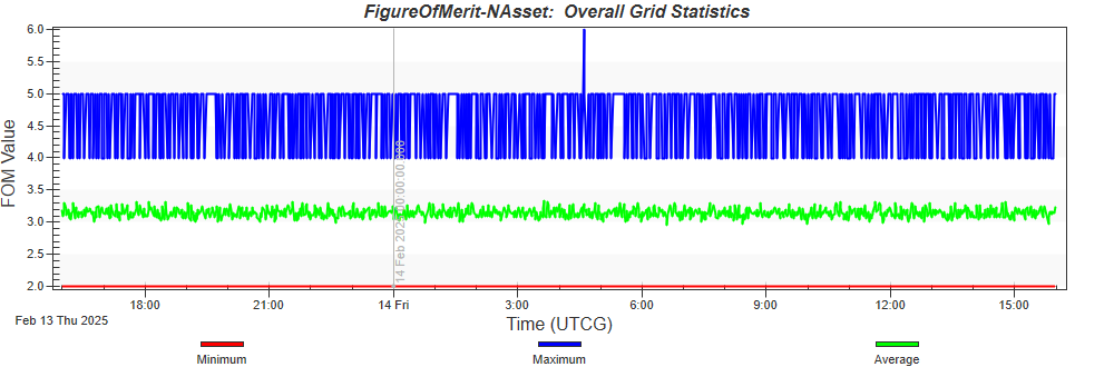
Grid stats over time graph
From these data, you can see that you have full coverage throughout your mission. The minimum criterion of two satellites with simultaneous access to a grid point is met. This is confirmed in the Percent Satisfied Report and the Grid Stats Over Time graph. You can also see that you have a maximum of four to six satellites with simultaneous access to a grid point. This redundancy is key, in case you should lose a satellite in the course of a mission.
Your objective to create a new satellite constellation that provides persistent, stereo coverage of hypersonic vehicles across the world has been met.
Saving your work
Clean up your workspace and close out your scenario.
- When finished, close all tools, graphs and reports you still have open.
- Save () your work.
- Close the STK application.
Summary
You have the results of the optimization run, but there are many parameters that you can vary in the analysis. The flexibility of both the STK and the ModelCenter software enable you to change an aspect of the mission (like the semi-major axis) while knowing that it carries through and is used in all calculations. You can link your analysis into many other aspects of your model, incorporating cost breakdowns, the total number of satellites, and other parameters from many different, linked sources. You can thus integrate the mission earlier and take into consideration all of the factors in the mission environment.
DME Lesson 2: Hypersonics and EOIR
The next lesson in the DME series focuses on Hypersonics and EOIR. You will use a starter scenario and build your own hypersonic vehicle. You will use an EOIR sensor to image it. This leads up to sessions three and four of the DME series where you bring the constellation from this lesson and the flight from session two together to understand how all components for the mission works together.