STK Pro, STK Premium (Air), STK Premium (Space), or STK Enterprise
You can obtain the necessary licenses for this tutorial by contacting AGI Support at support@agi.com or 1-800-924-7244.
The results of the tutorial may vary depending on the user settings and data enabled (online operations, terrain server, dynamic Earth data, etc.). It is acceptable to have different results.
Capabilities Covered
This lesson covers the following STK Capabilities:
- STK Pro
- Communications
Problem Statement
A situation has arisen where two customers are utilizing a satellite communication downlink facility located in the Southwestern United States. One transmission is routine, but important. The other transmission is urgent.
There are only two satellite reception parabolic antenna dishes available and they sit next to each other. Although the communications are coming from different locations, they are being routed through the same satellite to the ground facility.
Break It Down
You have some information that may be helpful. Here’s what you know:
- The communication satellite is geostationary.
- The satellite is transmitting two streams of data to the same ground site.
- The urgent communication link is transmitting on a frequency of 25 GHz.
- The routine communication link is transmitting on a frequency of 25.2 GHz.
- Both transmissions are using a data rate of 300 Mb/Sec.
- The close proximity of the frequencies, separated by 200 MHz, is causing interference with the data streams.
- As much as possible, you want to minimize interference without reducing bandwidth.
Solution
Using STK's Communications capability and RF spectrum filters, determine the filter and required settings that enable transmission reception.
Video Guidance
Watch the following video. Then follow the steps below, which incorporate the systems and missions you work on (sample inputs provided).
Open a Scenario
To speed things up and allow you to focus on the portion of this exercise that teaches you to create and display jammers in STK, a partially created scenario have been provided for you.
- Ensure that the Welcome to STK dialog box is visible in the STK Workspace.
- Click the Open a Scenario button.
- Browse to <Install Dir>\Data\Resources\stktraining\VDFs.
- Select Comm_RF_Spectrum_Filters.vdf (
 ).
). - Click Open.
- Open the File menu and select Save As.
- When the Save As window appears, click STK User.
- Click the Create New Folder icon.
- Rename the New folder RF_Filters.
- Select Comm_RF_Spectrum_Filters and click Open.
- Change File name: to RF_Filters.sc and click Save.
If using an older version of STK, browse to <Install Dir>\Data\Resources\stktraining\samples and open Comm_Filters.vdf.
When you open the scenario, a directory with the same name as the scenario will be created in the default user directory (C:\Users\<username>\Documents\STK_ODTK 13). The scenario will not be saved automatically.
When you save a scenario in STK, it will save in the format in which it originated. In other words, if you open a VDF, the default save format will be a VDF. The same is true for a scenario file (*.sc). If you want to save a VDF as a SC file (or vice-versa), you must change the file format when you are performing the Save As procedure.
Acquaint Yourself With the Scenario
You were provided a previously created scenario with all the objects needed for your analysis. You need to obtain situational awareness of the players in the scenario.
- Bring the 3D Graphics window to the front.
- Zoom To Urgent_Comms (
 ).
). - Mouse around in the 3D Graphics window to get a better view of the ground communication site.
- The antennas are oriented towards the communication satellite.
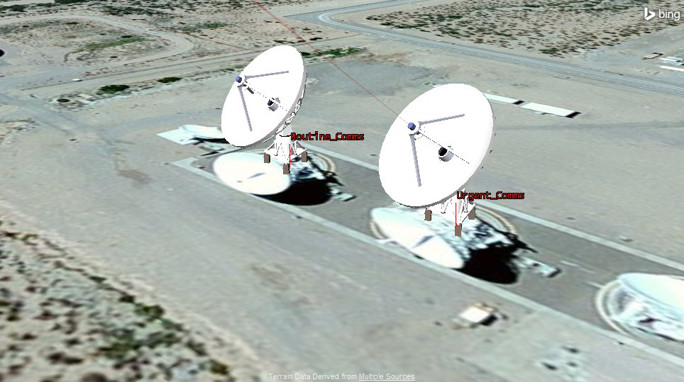
3D View: Communication ground site
Change Your Perspective
- Zoom To Tdrs3_19548 (
 ).
). - Mouse around in the 3D Graphics window to get a better view of the satellite antennas.
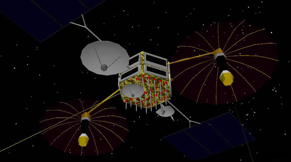
3D View: TDRS satellite antennas
You’ll notice the sensors for both transmitters are targeting the reception site on the ground. You may also notice that both transmitters are located on separate antenna locations on the satellite. The folding antennas are oriented toward the ground communication site.
Build the Constellations
Prior to analyzing filters, you need to double check if Urgent_Comms is being interfered with by Routine_Comms. You need to set up the three constellations (Receiver, Transmitter, Interference) to calculate interference. Begin with the receivers constellation.
Create the Receiver Constellation
- Using the Insert STK Objects tool, insert a Constellation object using the Define Properties method..
- On the Basic - Definition page, move (
 ) Urgent_Rcv (
 ) to the Assigned Objects list.
 - Click OK.
- Name the Constellation object Receiver.
Create the Transmitter Constellation
- Using the Insert STK Objects tool, insert a Constellation object using the Define Properties method.
- On the Basic - Definition page, move() Urgent_Xmt (
 ) to the Assigned Objects list.
 - Click OK.
- Name the Constellation object Transmitter.
Create the Interference Constellation
- Using the Insert STK Objects tool, insert a Constellation object using the Define Properties method.
- On the Basic - Definition page, move () Routine_Xmt () to the Assigned Objects list.
- Click OK.
- Name the Constellation object Interference.
Build the Comm System
Now that you have grouped the objects into constellations, you can build the CommSystem object.
- Using the Insert STK Objects tool, add a CommSystem (
 ) object to the scenario using the Insert Default method.
 - Open the CommSystem object's () properties (
 ).
). - On the Basic - Transmit page, move () the Transmitter constellation to the Selected Constellation column.
- Select the Receive page.
- Move () the Receiver constellation to the Selected Constellation column.
- Select the Interference page.
- Move () the Interference constellation to the Selected Constellation column.
- Click Apply.
If the Comm System object does not appear in the Insert Objects tool, click the Edit Preferences... button and add it.
Set the Time Step for the CommSystem
The default Start and Stop times for the CommSystem interval correspond to the scenario’s time period. You want the communication link to be calculated every 60 seconds, but the default step size is one (1) second.
- Select the Basic - Interval page.
- Set the Step Size to 60 sec.
- Click OK.
- Save (
 ) the scenario (
 ).
).
Calculating Interference
You’ll perform two calculations. The first is a graph depicting carrier wave interference. The second calculation is a detailed link budget.
- Select the CommSystem object() in the Object Browser.
- Click the Report & Graph Manager button (
 ) on the Data Providers toolbar.
 - Make the following changes:
| Option | Value |
|---|---|
| Show Reports | Off |
| Show Graphs | On |
Change the Carrier to Noise Graph Properties
Create a custom graph that represents the carrier to noise and carrier to noise with interference on the same axis. By default, they are on different axes.
- Select Carrier to Noise vs Time graph in the Installed Styles directory.
- Click the Properties () button.
- Move (
 ) the Link Information - C/(N + I) data provider from the Y2 axis.
 - Move () the Link Information - C/(N + I) data provider to the Y axis.
- Click OK.
- When the Information window appears, click OK.
- Expand the My Styles folder.
- Rename the graph My Carrier to Noise vs Time.
Generate the Graph
- Select My Carrier to Noise vs Time.
- Click Generate...
- Leave the graph open.
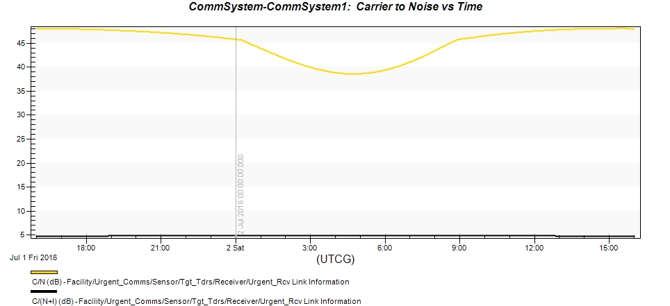
My Carrier to Noise vs Time
As you can see the line representing the clean carrier wave (C/N (dB)) and the line representing the wave that is receiving interference (C/N + I (dB)) are different. There is interference against the carrier wave.
Calculate the Link Budget
You have determined there is interference on the carrier wave, but sometimes with interference you can still communicate. Determine how good the quality of the communication is by looking at the Bit Error Rate (BER).
- Bring the Report & Graph Manager to the front.
- Make the following changes:
- Click Generate...
- Locate the BER and BER+I columns. The BER column shows the link performance without interference while the BER + I shows the link performance with interference.
- Can you see how interference is affecting your link?
- Leave the report open.
| Option | Value |
|---|---|
| Show Reports | On |
| Show Graphs | Off |
| Style | Link Information - Detailed |
| Generate as | Report/Graph |
When you compare the BER values with and without interference, you can see that interference has a major impact on the communications.
You can use this Link Information - Detailed report throughout the analysis to see how filtering affects the link.
Power Spectral Density
You have determined that there is considerable interference being caused by both transmissions in close proximity to each other. The engineering team has been tasked to model the filtering and mitigate the interference.
Bandwidth Analysis
The transmitted spectrum is modeled as a flat spectrum with unity magnitude across the transmitter’s bandwidth. The receiver’s frequency response is also modeled as a flat response across the receiver’s bandwidth. Therefore, the bandwidth ratio is computed as just a simple ratio of the receiver’s bandwidth to the transmitter’s bandwidth.
If the transmitter’s bandwidth is totally contained within the receiver’s bandwidth, the ratio will be one (1.0). For a receiver that has an auto scaled bandwidth and an auto tracked frequency, this value will be one (1). Otherwise, the value may be less than one (1.0) if the receiver center frequency and the transmitter frequency are not the same or the receiver’s bandwidth is totally contained within the transmitter’s bandwidth.
- Bring the Link Information - Detailed report to the front.
- Locate the Bandwidth (MHz) and Bandwidth Overlap (units) columns.
Note that the Bandwidth Overlap is one (1.0). This shows that you are capturing all the energy from the transmitted signal at the receiver.
The bandwidth is 300 MHz, which is what it should be.
Change the Receiver’s Bandwidth
Before using filters, experiment and change the receiver’s bandwidth to determine the effect that change might have on signal quality. Remember, the smaller the bandwidth, the less information that can be sent or received.
- Open Urgent_Rcv’s () properties ().
- Select the Basic - Definition page.
- Select the Filter tab.
Auto Scale
The Bandwidth Auto Scale option is available for the noise equivalent bandwidth of the receiver. This feature allows the receiver to adjust its bandwidth to that of the current transmitter as you switch from one transmitter to another. Since you’re receiving from a transmitter utilizing a bandwidth of 300 MHz, the receiver will automatically adjust with this option enabled.
- Disable the Auto Scale option.
- Set the Bandwidth to 150 MHz. That is half the transmitter’s bandwidth.
- Click OK.
- Refresh the Link Information Detailed report.
- What is the Bandwidth Overlap?
- Did the Bandwidth Overlap change?
- If so, by how much?
Theory
The Power Spectral Density (PSD), which describes how the power of a signal or time series is distributed with frequency. Here power can be the actual physical power, or more often, for convenience with abstract signals, can be defined as the squared value of the signal. This assumes the actual power of a signal is a 1-ohm voltage load.
The units of power spectral density are commonly expressed in watts per hertz (W/Hz). A spectral filter allows only a specific bandwidth of the electromagnetic spectrum to pass.
Signal PSD
Up until now, the power has been spread equally across frequency bands. In reality, the power is concentrated around the band center. Power Spectral Density allows you to model the reality case.
The PSD option allows the scenario to model the actual spectral shape of the transmitted signal based on the modulation, data rate, etc.
The Use Signal PSD option uses the modulation’s power spectral density to determine the Bandwidth Overlap Factor. If this option is not selected, the PSD will be modeled as a flat spectrum with unity magnitude across the transmitter’s bandwidth.
You have modeled a flat signal magnitude over the entire bandwidth which is sufficient fidelity for most conventional analysis. You are going to increase the fidelity by applying the appropriate signal shape over the entire bandwidth based on the modulation type.
You can apply filters to enhance the magnitude over certain frequencies content while suppressing the magnitudes over other frequencies. The use of Spectral Filters on transmitters modifies the spectral shape. The use of Spectral Filters on receivers helps reduce the impact of out of band signals from jammers and other sources.
- Open Routine_Xmt’s () properties ().
- Select the Basic - Definition page.
- Select the Modulator tab.
- Enable the Use Signal PSD option.
- Click OK.
The Use Signal PSD uses the modulation’s power spectral density to determine the Bandwidth Overlap Factor. If this option is not selected, the PSD will be modeled as a flat spectrum with unity magnitude across the transmitter’s bandwidth.
Enable PSD for the Transmitter
- Follow the same steps to enable Use Signal PSD for Urgent_Xmt.
- Bring the Carrier to Noise vs Time graph to the front.
- Refresh the graph.
- Can you still see interference to the carrier wave?
- Close the My Carrier to Noise vs Time Jam graph.
Check the Bandwidth Overlap Factor
Let’s check the Bandwidth Overlap Factor now that you have enabled Signal PSD.
- Bring the Link Information - Detailed report to the front.
- Refresh the report.
- Locate the Bandwidth Overlap column.
- Does the bandwidth overlap?
- If so, how much?
Notice the Bandwidth Overlap is ~0.78, which is greater than when the Use Signal PSD was disabled for the same bandwidth. The Spectral Power is spread over an infinite bandwidth - more densely towards the center of the band than at the band edges. In the Use Signal PSD enabled case, the power is spread over a wider range and the 150 MHz receiver captures approximately 78% of the signal instead of 50% when it was disabled.
Change the Modulation Type
One way to minimize bandwidth costs is to change the modulation to Phase Shift Keying with 16 Constellation Points (16PSK). Change the modulation to 16PSK and see if this has an effect on your signal quality.
- Open Urgent_Xmt’s () properties ().
- Select the Basic - Definition page.
- Select the Modulator tab.
- Set the Modulation Type to 16PSK.
- Enable the Use Signal PSD option.
- Click Apply.
- Refresh the Link Information Detailed report.
- Does the bandwidth overlap?
- If so, how much?
Notice that changing the modulation to 16PSK has nearly the same effect as increasing the receiver bandwidth to 300 MHz with QPSK modulation. 16PSK has a bandwidth ratio of 0.5 Hz/bps. QPSK has a bandwidth ratio of one (1.0) Hz/bps.
Reset the Transmitter’s Modulation
Return the transmitter’s modulation back to QPSK.
- Bring Urgent_Xmt’s () properties () to the front.
- Select the Basic - Definition page.
- Select the Modulator tab.
- Set the Modulation Type to QPSK.
- Enable the Use Signal PSD option.
- Click OK.
Reset the Receiver’s Auto Scale
- Open Urgent_Rcv’s () properties ().
- Select the Basic - Definition page.
- Select the Filter tab.
- Enable the Auto Scale option.
- Click OK.
- Refresh the Link Information Detailed report.
Spectrum and Filter Graph
The first filter you will use is the Butterworth filter. You will run a spectrum and filter graph to determine the cutoff frequency of the interference transmitter (Noise_Xmt). Using the graph, you’ll enable the Butterworth filter to see how it affects the link.
- Bring the Report & Graph Manager () to the front.
- Make the following changes:
- Click Generate...
- Right-click inside the graph.
- Select Grid Options.
- Select Show X Axis Grid Lines.
| Option | Value |
|---|---|
| Object Type | Transmitter |
| Object (Below Object Type) | Satellite/Tdrs3_19548/Sensor/Tgt_Uc/Urgent_Xmt |
| Show Reports | Off |
| Show Graphs | On |
| Style | Transmitter Spectrum and Filter |
| Generate as | Report/Graph |
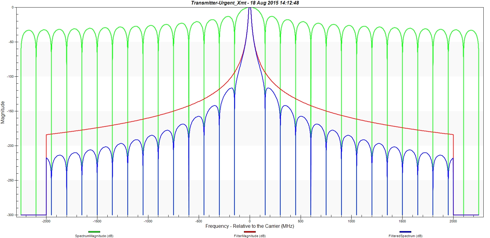
![]()
Transmitter Spectrum
Looking at the graph, you can see the bandwidth encompasses 4500 MHz. The main beam is 300 MHz.
Butterworth Filters
The filter cutoff frequency controls where you want the signal to start being suppressed and the filter order (rolloff) controls how steep you want the filter magnitude to drop or how fast you want the signal to get suppressed.
The Butterworth filter is less complex and maintains a flat profile over the filter bandwidth, but doesn’t have as steep a rolloff as Chebyshev. However, the Chebyshev is more complex and uses recursive equations (not a closed formula) and there is a ripple in the passband. This means you do not have a flat profile over the filter bandwidth. The Butterworth filter has a frequency response with flat pass and stop bands.
- Open Urgent_Xmt’s () properties ().
- Select the Basic - Definition page.
- Select the Filter tab.
- Enable the Use option.
- Ensure the Butterworth Filter is enabled.
- Set the following options:
- Click Apply.
- Refresh the Transmitter Spectrum and Filter graph.
| Option | Value |
|---|---|
| Upper Bandwidth Limit | 2000 MHz |
| Lower Bandwidth Limit | -2000 MHz |
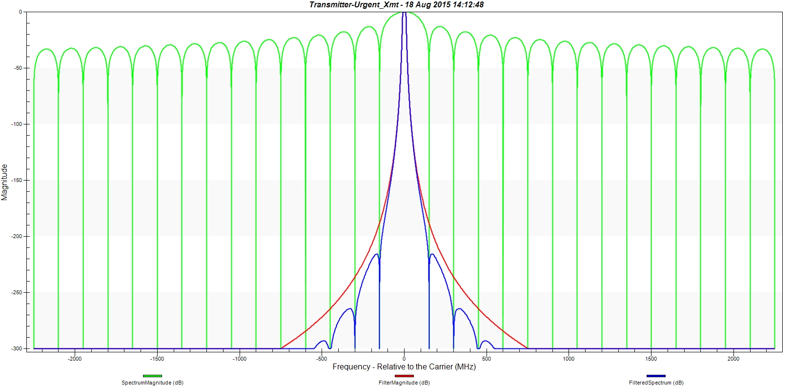
Transmitter and Spectrum Filtering with Butterworth
You have removed 500 MHz of bandwidth. Using the default frequency cutoff, you’ve narrowed the cutoff at ten (10) MHz on both sides of the carrier wave. You can see from the graph that the bandwidth has been suppressed on both sides of the carrier wave. Let’s see how this affects the BER.
Refresh the Link Information Detailed Report
- Bring the Link Information - Detailed report to the front.
- Refresh the report.
- Locate the BER + I column.
- Did you remove some interference?
- Are your BER + I rates better or worse?
Although your filter is working, you now have a new problem. You caused the BER to drop below acceptable levels during periods of your analysis. You have increased the BER with interference as well. This indicates your communication link is still poor.
Change the Filter Order
You would like to have a steeper roll off at the cutoff frequency. To ensure the filter has a steeper roll off, you can increase the filter order.
- Bring Urgent_Xmt’s () properties () to the front.
- Select the Basic - Definition page.
- Select the Filter page.
- Set the Filter Order to 8.
- Click Apply.
- Refresh the Transmitter Spectrum and Filter graph.
Butterworth with higher Frequency Order
You will notice the steep roll off in the filter profile. The steeper the roll off the better, but there are tradeoffs. One tradeoff is the steeper the roll off, the more complex the filter function. The more complex the filter function, the harder it is to implement, due to the complexity.
Refresh the Link Information Detailed Report
- Bring the Link Information - Detailed report to the front.
- Refresh the report.
- Locate the BER + I column.
- Did you notice an increase in BER + I values?
The change is minimal but the BER + I is still too high.
Change the Cutoff Frequency
Earlier, you determined that your center beam is 300 MHz wide. Your frequency cutoff is only ten (10) MHz. Widen the cutoff to -100 MHz to 100 MHz (200 MHz).
- Bring Urgent_Xmt’s () properties () to the front.
- Select the Basic - Definition page.
- Select the Filter page.
- Set the Cut-off Frequency to 100 MHz.
- Click Apply.
- Refresh the Transmitter Spectrum and Filter graph.
- Can you see how your filter is allowing more bandwidth through?
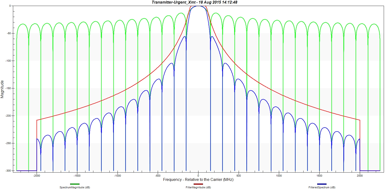
Butterworth with Cutoff Frequency
Refresh the Link Information Detailed Report
- Bring the Link Information - Detailed report to the front.
- Refresh the report.
- Locate the BER + I column.
- Did you notice an decrease in BER + I values?
Interference (BER + I) is still affecting the link.
Chebyshev Filter
The Chebyshev filter has a frequency response with equal ripple in the pass band.
- Bring Urgent_Xmt’s () properties () to the front.
- Select the Basic - Definition page.
- Select the Filter tab.
- Select Chevbyshev as the Filter Type.
- Set the following options:
- Click OK.
- Refresh the Transmitter Spectrum and Filter graph.
- Do you notice the five (5) dB ripple in the filter and filtered spectrum?
| Option | Value |
|---|---|
| Upper Bandwidth Limit | 2000 MHz |
| Lower Bandwidth Limit | -2000 MHz |
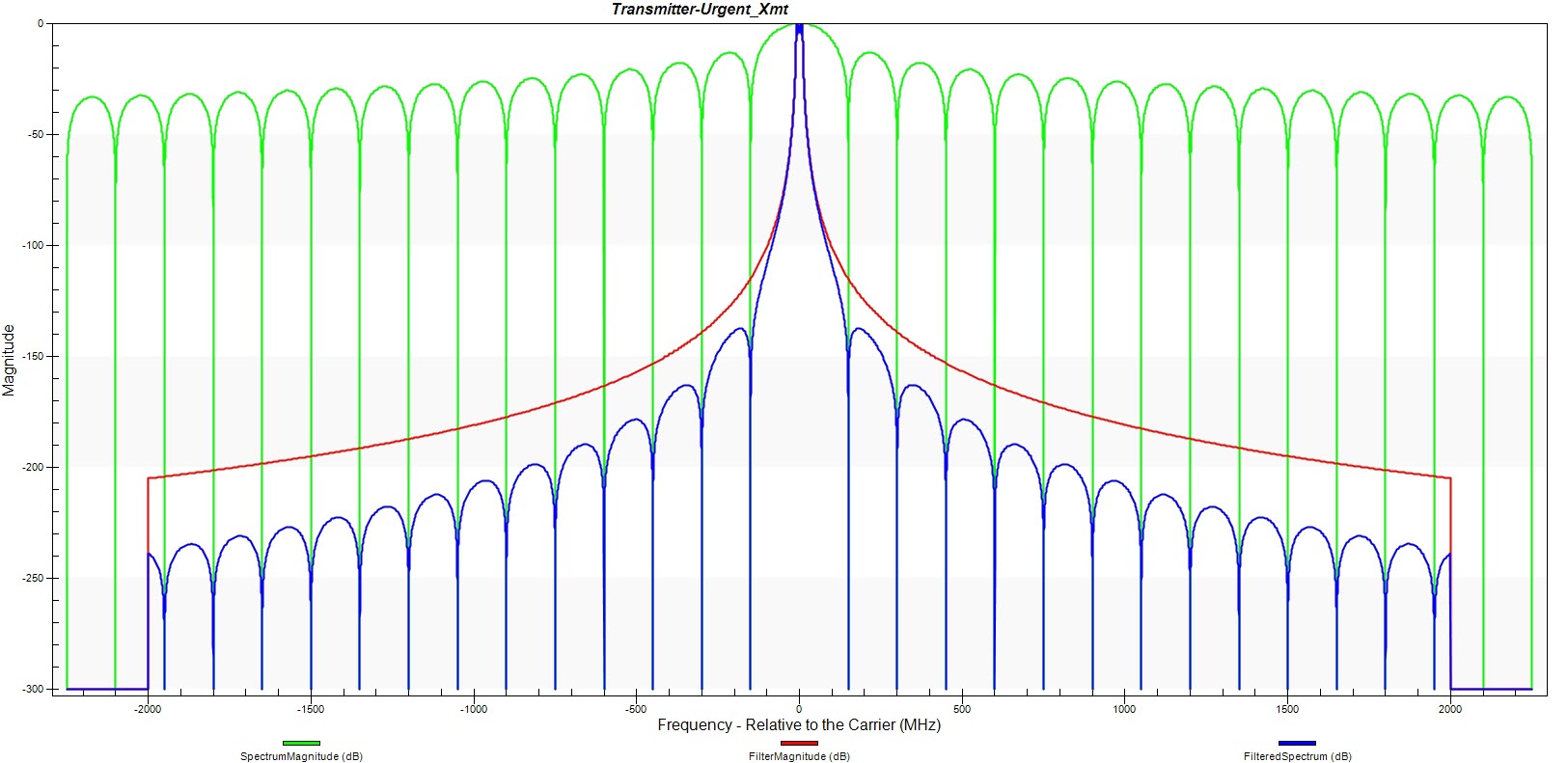
Chebyshev Filter
Refresh the Link Information Detailed Report
- Bring the Link Information - Detailed report to the front.
- Refresh the report.
- Locate the BER + I column.
- Did you notice an increase in BER + I values?
- Close the Transmitter Spectrum and Filter graph.
It’s time to apply a filter to the receiver.
Graph the Receiver Filter
- Bring the Report & Graph Manager () to the front.
- Set the Object Type to Receiver.
- Select Facility/Urgent_Comms/Sensor/Tgt_Tdrs/Urgent_Rcv.
- Select Receiver Filter graph style.
- Generate the graph.
- Right-click inside the graph.
- Select Grid Options.
- Right click on the graph, click Grid Options, and select Show X and Y Axis Grid Lines.

No Receiver filtering
Currently, you are not using a filter, so there is no effect against the receiver.
Apply the Chebyshev Filter to the Receiver
You tried both filters on the transmitter, let’s try the Chebyshev filter on the receiver. Then you see what effect the filter might have on the communication link.
- Open Urgent_Rcv () properties ().
- Select the Basic - Definition page.
- Select the Filter tab.
- Enable the Filter Model - Use option.
- Select Chevbyshev as the Filter Type.
- Set the following options:
- Click Apply.
- Refresh the Receiver Filter graph.
- Do you notice the five (5) dB ripple in the filter and filtered spectrum?
| Option | Value |
|---|---|
| Upper Bandwidth Limit | 2000 MHz |
| Lower Bandwidth Limit | -2000 MHz |
| Cut-off Frequency | 100 MHz |
| Ripple | 5 dB |

Chebyshev receiver Cutoff Frequency
You can see how the filter is suppressing noise on both sides of the carrier wave.
Change the Receiver Filter to a Butterworth
- Bring Urgent_Rcv () properties () to the front.
- Select the Basic - Definition page.
- Select the Filter tab.
- Select Butterworth as the Filter Type.
- Set the following options:
- Click OK.
- Refresh the Receiver Filter graph.
- Close the Receiver Filter graph.
| Option | Value |
|---|---|
| Upper Bandwidth Limit | 2000 MHz |
| Lower Bandwidth Limit | -2000 MHz |
| Cut-off Frequency | 10 MHz |

Butterworth Receiver Cutoff Frequency
You can see that the ripple disappears and the frequency cutoff isn’t so steep. Apply the Butterworth filter to Urgent_Xmt.
Set the Filter for the Transmitter
You can apply the Butterworth filter to the transmitter to try and improve performance even more.
- Open Urgent_Xmt’s () properties ().
- Select the Basic - Definition page.
- Select the Filter tab.
- Enable the Use option.
- Set the Filter to Butterworth.
- Set the following options:
- Click OK.
| Option | Value |
|---|---|
| Upper Bandwidth Limit | 2000 MHz |
| Lower Bandwidth Limit | -2000 MHz |
| Cut-off Frequency | 100 MHz |
Refresh the Link Information Detailed Report
- Bring the Link Information - Detailed report to the front.
- Refresh the report.
- Locate the BER + I column.
- Did your communication link improve?
- Do you still have interference?
- Are the BER + I values acceptable?
- Locate the Bandwidth Overlap (units) column
- Did bandwidth overlap decrease?
You have determined that you will need to filter both the transmitter and the receiver in order to minimize interference on your communication link. The Chebyshev filter removes the greatest amount of interference, but it increases the BER values.
The Butterworth filter decreases the BER values, but there’s a bit more interference in the communication link. Both filters require you to decrease bandwidth and the amount of information that can be transmitted over the communication link.
Save Your Work
- Close the Link Information - Detailed report.
- Close the Report & Graph Manager ().
- Save () your work.