STK Premium (Air), STK Premium (Space), or STK Enterprise
You can obtain the necessary licenses for this tutorial by contacting AGI Support at support@agi.com or 1-800-924-7244.
Required Capability Install: For versions 12.10 and earlier of the STK software, this lesson requires the installation of the EOIR capability. For these versions of the software, the EOIR installer is included in the STK Premium software download, but requires a separate installation process. Read the Readme.htm found in the STK software install folder for installation instructions. You can obtain the necessary install by visiting https://support.agi.com/downloads or calling AGI support.
The results of the tutorial may vary depending on the user settings and data enabled (online operations, terrain server, dynamic Earth data, etc.). It is acceptable to have different results.
Capabilities covered
This lesson covers the following capabilities of the Ansys Systems Tool Kit® (STK®) digital mission engineering software:
- STK Pro
- Electro-Optical Infrared Sensor Performance (EOIR)
Problem statement
Engineers and analysts need to quickly determine when a system can detect, track, identify, and characterize targets of interest under operational conditions. Modeling and simulating these system behaviors is critical to the success of a mission, and results support concept design, engineering, test, and operations. You want to model a geosynchronous satellite with optical sensors and the cloud patterns it would see from orbit. You also want to observe the results in the sensor data. Going forward, you can then account for potential targets becoming obscured.
Solution
Use the STK software's Electro-Optical Infrared Sensor Performance (EOIR) capability to model the detection, tracking, and imaging performance of electro-optical infrared (EOIR) sensors and account for time-dynamic clouds — the natural enemy of all optical systems — in your mission.
What you will learn
Upon completion of this tutorial, you will be able to:
- Design a space-based EOIR weather observation system
- Visualize clouds in the 2D and 3D Graphics windows
- Incorporate clouds into EOIR sensor scenes
- Calibrate an EOIR sensor when viewing clouds
Creating a new scenario
First, you must create a new scenario, then build from there.
- Launch the STK application (
 ).
). - Click
 Create a Scenario in the Welcome to STK dialog box.
 - Enter the following in the STK: New Scenario Wizard:
- Click when you finish.
- Click Save (
 ) when the scenario loads.
 - Verify the scenario name and location when the Save As dialog box opens.
- Click .
| Option | Value |
|---|---|
| Name | EOIR_CloudPatterns |
| Start | Default |
| Stop | Default |
A folder with the same name as your scenario is created for you.
Save () often during this lesson!
Disabling streaming terrain
By default, the STK application connects to the Ansys Geospatial Data Cloud to distribute Earth terrain data for analysis and visualization. Turn off
- Right-click on EOIR_CloudPatterns () in the Object Browser.
- Select Properties (
 ) in the shortcut menu.
 - Select the Basic - Terrain page when the Properties Browser opens.
- Clear the Use terrain server for analysis check box in the Terrain Server panel.
- Click to confirm your change and to close the Properties Browser.
Inserting a Facility object
Use a
- Bring the Insert STK Objects tool (
 ) to the front.
 - Select Facility (
 ) in the Select An Object To Be Inserted list.
 - Select Insert Default () in the Select A Method list.
- Click .
- Right-click on Facility1 () in the Object Browser.
- Select Rename in the shortcut menu.
- Rename Facility1 () GroundSite.
Inserting a Satellite object
Build the Earth observation satellite by inserting a new
- Bring the Insert STK Objects tool () to the front.
- Insert a Satellite (
 ) object using the Orbit Wizard (
 ) method.
 - Open the Type drop-down list when the Orbit Wizard opens.
- Select Geosynchronous.
- Enter EarthObsSat in the Satellite Name field.
- Select the Show All Objects check box in the Graphics panel.
- Enter -75 deg in the Subsatellite Point field in the Definition panel.
- Leave the Inclination set to 0 deg.
- Click to propagate EarthObsSat () and to close the Orbit Wizard.
Showing all objects helps you see where GroundSite is with respect to the satellite. Since the satellite is in GEO, as long as you are on the correct side of the hemisphere, you are able to see GroundSite.
Configuring the space-based sensor
You are creating a space-based Earth observation system.
Inserting a Sensor object
Insert a
- Bring the Insert STK Objects tool () to the front.
- Insert a Sensor (
 ) object using the Define Properties () method.
 - Select EarthObsSatellite () when the Select Object dialog box opens.
- Click to confirm your selection and to close the Select Object dialog box.
Defining the sensor Pointing properties
By default, the sensor is mounted on the satellite with a Fixed
- Select the Basic - Pointing page when the Properties Browser opens.
- Open the Pointing Type drop-down list.
- Selected Targeted.
- Select GroundSite () in the Available Targets list in the Targeted panel.
- Move (
 ) GroundSite () to the Assigned Targets list.
 - Click to confirm your changes and to keep the Properties Browser open.
Configuring an EOIR sensor
You've defined the pointing behavior of the sensor. Next, you can build the electro-optical infrared components of your mission. The STK software's Electro-Optical Infrared Sensor Performance (EOIR) capability models the detection, tracking, and imaging performance of electro-optical and infrared sensors. With the EOIR capability, you can generate accurate imagery and system-to-target metrics across ultraviolet, visible, and infrared wavelengths (0.28 to 28 microns).
Selecting the EOIR sensor definition
To create an EOIR scene, you need to specify the EOIR properties for the sensor and the other objects in the scenario. Start with the sensor. Select EOIR for the sensor's
- Select the Basic - Definition page.
- Open the Sensor Type drop-down list.
- Select EOIR.
- Click to confirm your changes and to keep the Properties Browser open.
Configuring the EOIR spatial properties
When you select an EOIR as the Sensor Type, you can select the Spatial tab to specify the
- Select the Spatial tab.
- Note that by default, a single band will be rendered.
- Leave the Input set to Field-of-View and Number of Pixels.
- Enter the following values in the Field of View panel:
- Enter the following values in the Number of Pixels panel:
- Click to confirm your changes and to keep the Properties Browser open.
You can choose which two optical parameters are used as inputs, used to calculate a third parameter — in this case, the detector pitch will be calculated.
| Option | Value |
|---|---|
| Horizontal Half Angle | 5 deg |
| Vertical Half Angle | 5 deg |
The EOIR capability uses these values to determine the full angular extent of the sensor's field of view.
| Option | Value |
|---|---|
| Horizontal | 200 |
| Vertical | 200 |
These are the number of sensor pixels in the field of view in the horizontal and vertical directions; the default is 128 for each.
Configuring the EOIR spectral properties
Your sensor analyzes the visible waveband between 0.4 to 0.7 microns. Confirm the sensor is configured for visible light by reviewing the spectral band edge definitions in the sensor's
- Select the Spectral tab.
- Locate the Spectral Band Edge Wavelengths panel.
- Confirm that Low is set to 0.400000 (um).
- Confirm that High is set to 0.700000 (um).
Low is the shortest wavelength that the sensor responds to. High is the longest wavelength to which the sensor responds.
Configuring the EOIR optical properties
Configure the sensor's
- Select the Optical tab.
- Open the Input drop-down list.
- Select F-Number and Entrance Pupil Diameter.
- Leave the F/# set to the default value of 2.000000.
- Enter 100 in the Entrance Pupil Diameter field.
- Open the input drop-down list in the Image Quality panel.
- Select Negligible Aberrations.
- Click to confirm your changes and to keep the Properties Browser open.
This is the Effective Focal Length/Effective Pupil Diameter of the optical prescription.
This is the diameter (in centimeters) of the "single-lens equivalent" optical prescription. 100 centimeters is considered commercially viable.
The EOIR capability models aberrations based on a root-mean-square(RMS) wavefront error; for negligible aberrations, the RMS wavefront error is equal to 0.07.
Configuring the EOIR radiometric properties
Update the sensor's
- Select the Radiometric tab.
- Ensure the Input is set to High Level.
- Click to confirm your selection and to close the Properties Browser.
- Rename Sensor1 () EOIR_Visible.
At a high level, the sensitivity defines the noise floor of the sensor. After generating the sensor scene, you can revisit these parameters.
Opening the EOIR toolbar
Use the  ) to access the EOIR configuration and EOIR sensor scene for a particular sensor.
- Select the View menu in the Menu Bar.
- Select the Toolbars menu.
- Select EOIR in the Toolbars submenu.
Generating an EOIR sensor scene
Use the EOIR capability's
- Select EOIR_Visible () in the Object Browser.
- Click EOIR Sensor Scene... (
 ) on the EOIR toolbar to generate an image that represents the sensor output.
Updating the EOIR scene visual details
An EOIR sensor scene's
- Right-click in the EOIR Sensor Scene window after it is generated.
- Select Details... in the shortcut menu.
- Select the Fine option in the Scene Detail panel when the EOIR Scene Visual Details dialog box opens.
- Click to confirm your selection and to close the EOIR Scene Visual Details dialog box.
- Review the sensor scene.
- Close the EOIR Sensor Scene window.
The scene is initially generated to the spatial resolution of the tessellations. When you use a Fine detail, further calculations apply image interpolation algorithms that smooth off the edges of the tessellations.
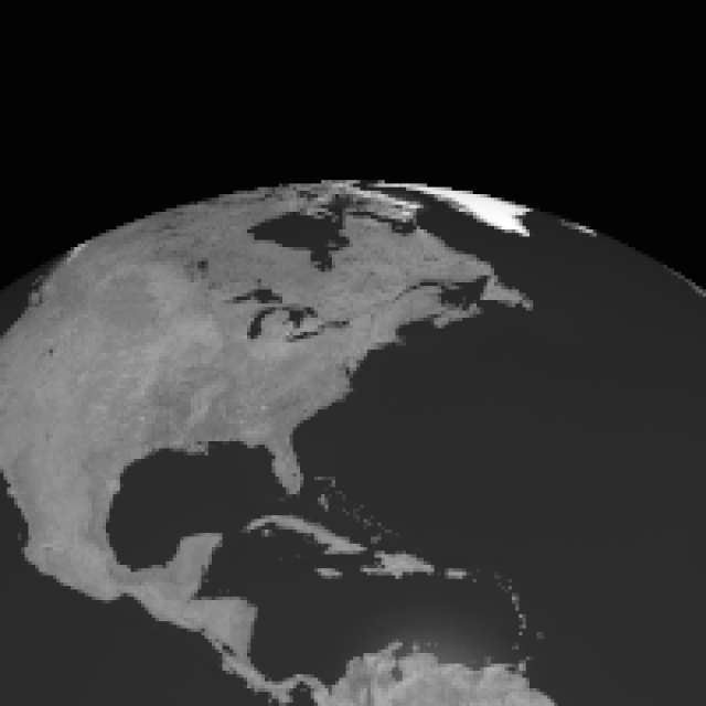
EOIR sensor scene without clouds
The current state of the Earth is without any visible weather patterns — that is, clouds. In order to view them in the sensor scene, you must first account for them in the EOIR configuration.
Visualizing clouds in the 3D and 2D Graphics windows
Before loading clouds analytically into an EOIR sensor scene, it is helpful first to visualize what you should expect to see in the 3D and 2D Graphics windows.
Visualizing clouds with the Globe Manager
You can use the
- Bring the 3D Graphics window to the front.
- Click Globe Manager (
 ) on the 3D Graphics window's Globe Manager toolbar.
 - Select the Clouds.cld (
 ) check box in the Globe Manager Hierarchy when the Globe Manager Hierarchy window opens.
The .cld file extension is shorthand for cloud. Clouds.cld is part of the STK software installation and is located in <Install Dir>\STK_ODTK 13\STKData\VO\Clouds. You can open this file in a text editor of your choice, such as Notepad or Notepad++. It contains a starting datetime and the name of the cloud map, which can be in a variety of formats (for example, *.png, *.pgm, *.jpg., etc.) Datetime stamps, which increase stepwise, create a dynamic cloud model with corresponding images in the scenario.
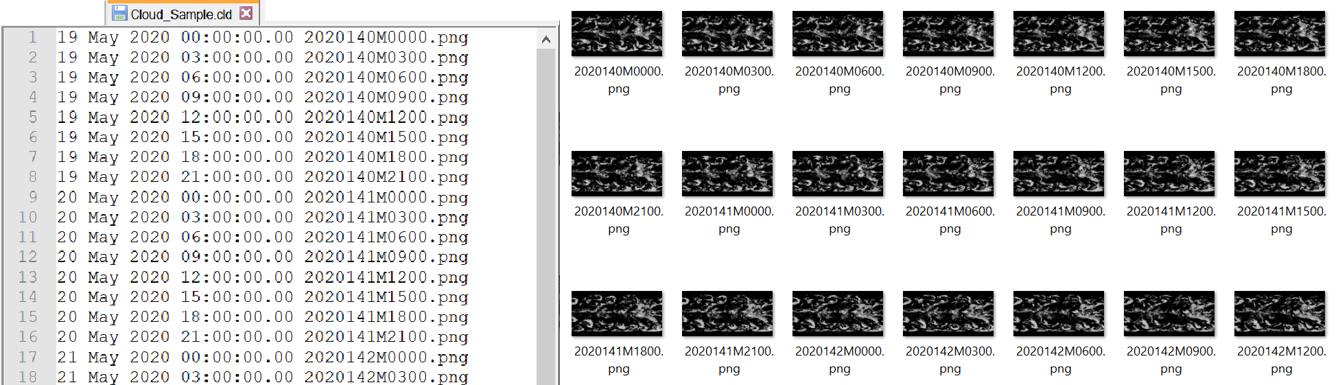
example cloud file contents (left) and the associated series of images (right)
The Clouds.cld cloud file contains a single line referencing a single portable gray map image file, Clouds.pgm, which is also included with the STK software installation. Using Clouds.cld, your cloud model will remain static.
Updating the cloud file's properties
You can also change the altitude at which the cloud layer is visualized.
- Right-click on Clouds.cld ().
- Select Properties... () in the shortcut menu.
- Enter 10 km in the Altitude field when the Globe Manager: Cloud Properties dialog box opens.
- Click to confirm your change and to close the Globe Manager: Cloud Properties dialog box.
Viewing the clouds in the 3D Graphics window
With your cloud altitude configured, view the results in the 3D Graphics window.
- Clear the check box for EOIR_Visible () in the Objects Browser to get a better look at the clouds.
- Examine the clouds in the 3D Graphics window.
- Select the check box for EOIR_Visible () in the Objects Browser to turn the display of the sensor back on.
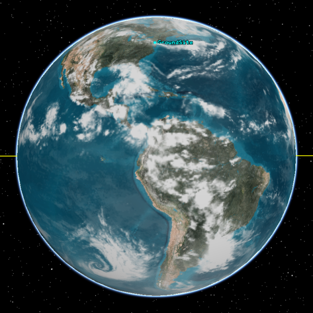
Clouds in the 3D Graphics window
This gives you an idea of what you should see in the EOIR sensor scene.
Visualizing clouds in the 2D Graphics window
You can also overlay images of clouds in the 2D Graphics window by updating the
- Bring the 2D Graphics window to the front.
- Click Properties () on the 2D Graphics window's 2D Window Defaults toolbar.
- Select the Details page when the Properties Browser opens.
- Select the Cloud File check box in the Clouds panel.
- Click the Cloud File ellipsis (
 ).
). - Navigate to the location of the installed Clouds.cld file at <Install Dir>\STK_ODTK 13\STKData\VO\Clouds when the Cloud File dialog box opens.
- Select Clouds.cld.
- Click to confirm your selection and to close the Cloud File dialog box.
- Click to confirm your changes and to close the Properties Browser.
- Examine the clouds in the 2D Graphics window.
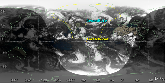
Clouds in the 2D Graphics window
Modeling clouds with the EOIR capability
You can choose to show
Updating the EOIR Configuration
Update the
- Click EOIR Configuration... (
 ) on the EOIR toolbar.
 - Click when the EOIR Configuration dialog box opens.
- Select the Clouds page when the EOIR Atmosphere, Clouds, and Texture Maps dialog box opens.
- Select the Show check box in the General panel.
Adding a cloud dataset
The Current Datasets panel displays all cloud datasets that are in the scenario. Add a sample cloud dataset to your EOIR configuration.
- Click .
- Enter Simple Clouds in the Dataset Label field.
- Enter 10.0000 in the Altitude field.
- Leave the Forward Scatter and Back Scatter fields set to 50.0000.
- Select the File option in the Coverage panel.
- Click the File ellipsis ().
- Select high_res_cloudmap.csv when the Open dialog box opens.
- Click to confirm your selection and to close the Open dialog box.
- Click to confirm your changes and to close the EOIR Atmosphere, Clouds, and Texture Maps dialog box.
- Click to confirm your changes and to close the EOIR Configuration dialog box.
This specifies the height of the cloud layer above the ellipsoidal surface of the central body in kilometers. The limits are zero (0) km <= Altitude <= 100 km.
These specify the percentage of reflected incident solar illumination scattered to the opposite side of and back in the direction of the illumination source, respectively. The limits are 0% <= Front Scatter <= 100%.
For a file, you can select a clouds-only file (*.csv, *.cld, *.clds) or an image file (*.bmp, *.tif, *.png, *,jpg, *.ppm, *.pgm) to define the cloud coverage. Several sample CSV cloud files are available with the EOIR capability in <Install Dir>\STK_ODTK 13\EOIR_Databases\Clouds.
These cloud data are based on the Clouds.cld file.
Generating an EOIR sensor scene
EOIR can create an image of what the system on the EarthObsSat sees.
- Select EOIR_Visible () in the Object Browser.
- Click EOIR Sensor Scene... () on the EOIR toolbar to generate the sensor scene.
- Review the sensor scene.
- Close the EOIR Sensor Scene window.
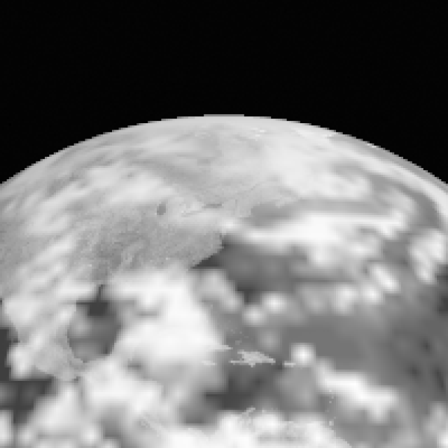
Visible Light EOIR sensor scene with clouds
Unlike before, you can now see clouds in your sensor scene.
Viewing Earth in the long-wavelength infrared band
The first EOIR sensor just looked at the visible part of the spectrum. Look at the long-wavelength infrared (LWIR) (8–15 microns). This is the thermal imaging region, or thermal infrared region, of the spectrum.
Reusing the Sensor object
You can reuse (copy and paste) the EOIR_Visible Sensor object, which is a quick way to create a new object having identical properties to an object already existing in the scenario.
- Select EOIR_Visible () in the Object Browser.
- Click Copy (
 ) on the Object Browser toolbar.
 - Select EarthObsSat () in the Object Browser.
- Click Paste (
 ) on the Object Browser toolbar.
 - Rename EOIR_Visible1 () EOIR_LWIR.
Updating the sensor's spectral properties
Update the sensor's spectral band edge wavelength bounds to focus on the LWIR region.
- Open EOIR_LWIR's () Properties ().
- Select the Basic - Definition page when the Properties Browser opens.
- Select the Spectral tab.
- Enter the following in the Spectral Band Edge Wavelengths panel:
- Click to confirm your changes and to keep the Properties Browser open.
- Save () your scenario.
| Option | Value |
|---|---|
| High | 15.000000 |
| Low | 8.000000 |
Set the high value first to keep all values within the limits.
Generating an EOIR sensor scene
Using the new sensor, generate a new sensor scene to see the differences in the model.
- Select EOIR_LWIR () in the Object Browser.
- Click EOIR Sensor Scene... () on the EOIR toolbar to generate a sensor scene.
- Right-click in the EOIR Sensor Scene window after the sensor scene is generated.
- Select Details... in the shortcut menu.
- Select the Fine option in the Scene Detail panel when the EOIR Scene Visual Details dialog box opens.
- Select the BGRY option in the Color Map panel.
- Review the sensor scene.
Color mapping is only for visual effect and does not change any of the internal data values.
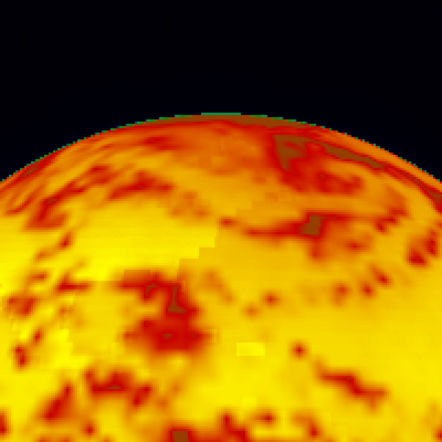
LWIR sensor scene
Viewing cloud inband radiance
The inband radiance order of magnitude gives you insight as to how the sensor's sensitivity should be configured.
- Click on an area of thick cloud cover in the EOIR sensor scene.
- Review the details in the Scene Pick Information panel in the EOIR Scene Visual Details dialog box.
- Take a look at the Inband Radiance value, specifically the order of magnitude.
The sensor's sensitivity can be adjusted to provide more detail.
Calibrating the LWIR sensor
Use the EOIR sensor scene to perform in-scene calibration of the LWIR sensor.
Selecting the units of saturation and sensitivity
Adjust the EOIR sensor's approach to saturation and sensitivity.
- Bring EOIR_LWIR's () Properties () to the front.
- Select the Radiometric tab.
- Select the Radiance (W/cm2 sr) option in the Units for Saturation and Sensitivity panel.
With the Radiance option, the Sensitivity and Dynamics Range parameters operate in radiance units (W∙cm-2∙sr-1). Radiance is better suited for sensors that are observing resolved images, where object shapes are discernible.
Defining the sensor's sensitivity and dynamic range
Adjust the sensor's sensitivity and dynamic range settings. Sensitivity defines the "noise floor" of the sensor; the Dynamic Range is the ratio of the brightest signal to the noise floor.
- Select the Simulate Saturation check box.
- Double-click on the EquivalentValue field in the Sensitivity panel.
- Enter 1e-05.
- Select the Enter key.
- Double-click on the EquivalentValue field in the Dynamic Range panel.
- Enter 0.3.
- Select the Enter key.
- Click to confirm your changes and to close the Properties Browser.
Selecting this check box allows the EOIR capability to simulate saturation, when pixels can only measure up to the specified saturation level of a radiant signal. This is the way physical detectors would behave. Saturation defines the "brightest" signal that the sensor can measure.
This is the Noise Equivalent Irradiance/Radiance (NEI/NER) vs. Integration Time. The sensor will not detect signals below this level. This value is found by varying the sensitivity until the sensor scene shows some noise in space, but otherwise a smoothed display.
This is the Saturation Equivalent Irradiance/Radiance (SEI/SER) vs. Integration Time. This value is found by varying the dynamic range.
Reviewing the calibrated EOIR sensor scene
The EOIR sensor scene will update automatically.
- Review the updated sensor scene.
- Click to close the EOIR Scene Visual Details dialog box.
- Close the EOIR Sensor Scene window.
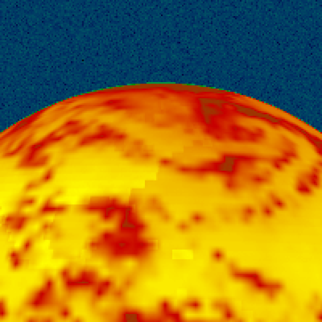
Calibrated LWIR sensor scene
Note that while there is more noise in space, the clouds appear smoother and are less saturated.
The EOIR capability processes the raw sensor data or a scene bitmap based on the selected level (radiometric input, geometric input, or sensor output) for each animation time step. Data from a sensor scene can be exported using the Automatic File Output panel in the EOIR Scene Visual Details dialog box. Post processing with Python and MATLAB allow you to analyze these results. Several example scripts for generating cloud data and analyzing the results are available on the AGI GitHub at
Saving your work
Clean up your workspace and save your work.
- Close any open tools, properties, and EOIR sensor scenes.
- Save () your work.
Summary
You began by configuring a sensor on a geostationary satellite. After configuring the sensor use the EOIR capability to view the visible range, you added a sample cloud file into your scenario for both visualization in the 3D Graphics window and for analysis in an EOIR senor scene. You then used another EOIR sensor to view the clouds in the LWIR spectrum range and calibrated the sensor's radiometric settings.
On your own
You can also turn clouds on and off in the EOIR configuration using the
EOIR */ SetAtmosphere Clouds On
EOIR */ SetAtmosphere Clouds Off
Additional cloud parameters can be set with Connect commands (for example, adding multiple cloud layers). To set cloud parameters via Connect, you can use the following syntax:
EOIR <ScenarioPath> CloudData SetValue <Label> <Parameter> <Value>
Valid values for Parameter are listed on the
EOIR */ SetAtmosphere Clouds On
EOIR */ CloudData DatasetTest1 0 1000
EOIR */ CloudData NewConstDataSet Test2
EOIR */ CloudData AddCldDataSets Test3 "...\CloudData.cld"