STK Premium (Air), STK Premium (Space), or STK Enterprise
You can obtain the necessary licenses for this tutorial by contacting AGI Support at support@agi.com or 1-800-924-7244.
Required product install: The Ansys ModelCenter® model-based systems engineering software and the STK Plugin for ModelCenter are required to complete this tutorial.
ModelCenter installation prerequisites: The ModelCenter software requires the installation of a 64-bit version of Java, a 64-bit implementation of Python 3.x, and the installation of the thrift and six Python packages. See the ModelCenter Installation Prerequisites for more information.
You should complete the Level 3 feature-specific tutorial Introduction to STK's Multifunction Radar prior to beginning this lesson in order to understand the STK software's multifunction radar properties and settings.
This tutorial was written using version 2026 R1 of the Ansys ModelCenter® model-based systems engineering software.
The results of the tutorial may vary depending on the user settings and data enabled (online operations, terrain server, dynamic Earth data, etc.). It is acceptable to have different results.
Capabilities covered
This lesson covers the following capabilities of the Ansys Systems Tool Kit® (STK®) digital mission engineering software:
- STK Pro
- Radar
- STK Analyzer
Problem statement
Engineers and operators employ multifunction radar (MFR) to track multiple types of targets. You want to track an aircraft, which is flying from an airbase in Spain, with a new MFR system located at its destination airbase in Italy. The terrain in the vicinity of the radar site must be accounted for analytically. You need a quick way to determine how various settings on the radar system will affect its ability to track the aircraft.
Solution
Use the STK application's Radar capability and the Analyzer capability, which is part of the Ansys ModelCenter® model-based systems engineering software, to examine various input variables and how they affect the multifunction radar's ability to track the aircraft.
What you will learn
Upon completion of this tutorial, you will have a basic understanding of the following:
- How to analyze a multifunction radar with the ModelCenter software
- How an MFR's gain, SNR, and integrated pulses affect its integrated probability of detection (PDet)
Using the starter scenario
To speed things up and allow you to focus on the portion of this exercise that teaches you how to use the ModelCenter software, a partially created scenario has been provided for you.
Opening the starter scenario
The starter scenario is included in your install.
- Launch the STK application (
 ).
). - Click
 Open a Scenario in the Welcome to STK dialog box.
 - Browse to <Install Dir>\Data\Resources\stktraining\VDFs.
- Select MFR_Analyzer_Starter.vdf.
- Click .
Saving the VDF as a scenario file
Save and extract the VDF data in the form of a scenario folder. When you save a VDF in the STK application, it will save in its originating format. That is, if you open a VDF, the default save format will be a VDF (.vdf). If you want to save and extract a VDF as a scenario folder, you must change the file format by using the Save As feature. This will create a permanent scenario file complete with child objects and any additional files packaged with the VDF.
- Open the File menu when the starter scenario opens.
- Select Save As....
- Select the STK User folder in the navigation pane when the Save As dialog box opens.
- Select the MFR_Analyzer_Starter folder.
- Click .
- Select Scenario Files (*.sc) in the Save as type drop-down list.
- Select the MFR_Analyzer_Starter scenario file in the file browser.
- Click .
- Click in the Confirm Save As Dialog box to overwrite the existing scenario file in the folder and to save your scenario.
A scenario folder with the same name as the VDF was created for you when you opened the VDF in the STK application. This folder contains the temporarily unpacked files from the VDF.
When saving a VDF as a scenario folder, you should extract its contents to the scenario folder the STK application automatically creates for you in the STK User folder. See the
Save (![]() ) often during this lesson!
) often during this lesson!
Reviewing the starter scenario
Use the set of three 2D and 3D Graphics windows to gain situational awareness of the aircraft's flight path and the test area.
- Look at the Aircraft 3D Graphics window, which is zoomed to the aircraft.
- Use your mouse to get an idea of where the aircraft is located and the airbase from which it just left.
- Click Start (
 ) in the Animation Toolbar to obtain situational awareness of the aircraft's location.
 - Adjust (
 ,
,  )the step size as desired.
 - When finished, Reset (
 ) the scenario.
 - Look at the Radar Site 3D Graphics window, which is zoomed to the radar site. The Radar_Site Place object and the attached MFR Radar object are both using an Az-El Mask constraint that takes into account the surrounding terrain.
- Look at the Flight Plan 2D Graphics window to obtain an overall view of the aircraft's flight path.
- Note the box located in northern Italy. The box is a visual representation of the analytical terrain boundaries. Everything outside the box is using the WGS84 altitude reference and everything inside the box uses analytical terrain (MFR_Terrain_Training.pdtt).
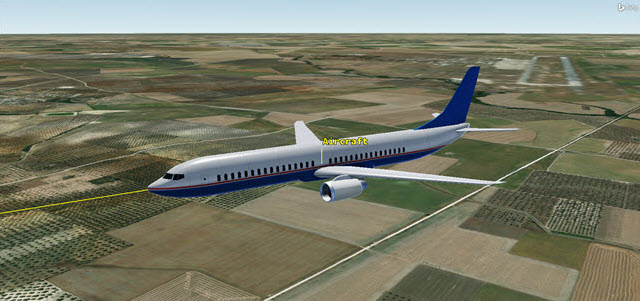
3D Graphics View of the Aircraft Leaving the Spanish Airbase
The aircraft is using a constant

3D Graphics View of the Radar Site and Surrounding Terrain
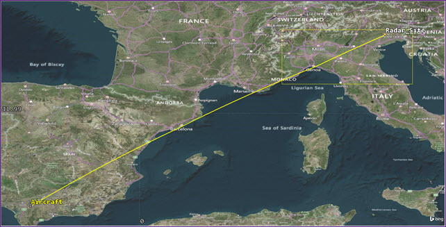
2D Graphics View of the Aircraft's Flight path
Understanding the MFR radar's properties
Prior to running any trade studies, you should understand the MFR's settings. The STK software's Radar capability provides thorough analysis and graphic displays of radar systems. It provides a Radar object that can be attached to an STK Vehicle, Facility, Place, Target, or Sensor object. The Radar object attached to Radar_Site, MFR, is a
Viewing the radar beam parameters
Open MFR's properties to review the beam specifications.
- Open MFR's (
 ) Properties (
 ).
). - Ensure the Beams tab is selected on the Basic - Definition page when the Properties Browser opens.
- Review the TargetTransport Beam ID in the beam summary table.
- Select the Beam Spec subtab.
- Note the Gain value of 30 dB. You will analyze this in the ModelCenter application.
Note the TargetTransport beam is targeting the aircraft.
Viewing the waveform strategy
Normally, you would want to use the Range setting for any target being tracked at different ranges. You are starting with a waveform strategy created for this analysis that is similar to the medium range rectangular strategy. Review the
- Select the Waveforms subtab.
- Note that the Waveform is set to MFR Analyzer Waveform.
- Click Component Browser (
 ).
). - Open the Show Component Type drop-down list.
- Select Radar Components.
- Select the Radar Waveforms (
 ) folder.
 - Double-click on MFR Analyzer Waveform (
 ) in the Radar Waveforms list.
 - Review the waveform settings.
- Click when finished.
- Close the Component Browser.
Understanding detection processing
The Detection Processing tab allows you to define probability of detection, pulse integration and pulse specifications.
- Select the Detection Processing tab.
- Select the Pulse Integration subtab.
- Note the integration method is set to Goal SNR.
- Click to close the Properties Browser without making any changes.
The Goal SNR integration method is based on the desired signal-to-noise ratio; its SNR value and the number of maximum pulses will be studied using the ModelCenter application.
Calculating access
Create an access between the radar and the aircraft. This is required prior to using the Report & Graph Manager and analyzing the MFR in ModelCenter.
- Right-click on MFR () in the Object Browser.
- Select Access... (
 ).
). - Select Aircraft (
 ) in the associated objects list when the Access Tool opens.
 - Click
 .
.
Reporting on the radar's effectiveness
The focus of this scenario is the Integrated PDet, which is the probability of detection integrated over the dwell of pulses. An Integrated PDet value of 0.8 to 1.0 is required to track the aircraft with certainty.
Creating a new report style
Create a custom report that provides pertinent data that will be analyzed when running the trade studies.
- Click below the Reports panel.
- Right-click on the MFR_Analyzer_Starter Styles () folder in the Styles panel when the Report & Graph Manager opens.
- Select New in the shortcut menu.
- Select Report (
 ) in the New submenu.
 - Enter Trade Study Data while in rename mode.
- Select the Enter key.
Defining the report content
You can define the contents and format of a new report style or modify the contents and format of an existing style. The properties available for defining the content and format of data will depend on the data providers in the selected report style. In this scenario, you are creating a custom report that contains elements of your choosing.
- Select the Content page when the Properties Browser opens.
- Delete the asterisk (*) in the Filter field.
- Enter Radar in the Filter field.
- Click .
- Expand (
 ) the Radar Multifunction (
 ) data provider in the Data Providers list.
 - Expand () the TargetTransport () data provider.
- Move (
 ) the following data provider elements (
 ) to the Report Contents field in the order shown:
- Time
- S/T Integrated SNR
- S/T Integrated PDet
- S/T Pulses Integrated
- Click to accept your changes and to close the Properties Browser.
Any beams that are added to the Beams list in the Radar object's properties will become a data provider under Radar Multifunction. TargetTransport is the default beam for this scenario.
Your custom report will include the signal-to-noise ratio over the dwell of pulses (S/T integrated SNR) and the number of pulses successfully integrated (S/T Pulses Integrated) over time, in addition to the Integrated PDet.
Generating the report
Now that you've built your custom report, generate it to review the results.
- Select Trade Study Data (
 ) in the MFR_Analyzer_Starter Styles () folder.
 - Click .
- Click at the top of the report.
- Change the Step to 10 sec.
- Click Refresh (F5) (
 ) in the report toolbar.
 - Scroll through the report until you find the first time S/T Integrated PDet is at or above 0.8.
- Look at the changes in S/T Integrated SNR (dB) and S/T Pulses Integrated throughout the report.
- Right-click on the time when the S/T Integrated PDet is first at or above 0.8.
- Select Time in the shortcut menu.
- Select Set Animation Time in the Time submenu.
You can use the data to determine how long the radar tracks the aircraft — starting at approximately nine minutes from the end of the scenario.
As the S/T Integrated PDet improves, S/T Integrated SNR (dB) increases and S/T Pulses Integrated decreases.
Obtaining situational awareness
With your animation time set to a period when the MFR can successfully begin tracking the aircraft, view your setup in the Radar Site 3D Graphics window.
- Bring the Radar Site 3D Graphics window to the front.
- Use your mouse to obtain a good view of the radar site and the beam pointing at the aircraft. The maximum gain is blue and minimum gain is red.
- Close the report, the Report & Graph Manager and the Access Tool when you are finished.
![]()
Radar Beam Tracking the Aircraft
Creating a new ModelCenter project
The
- Save (
 ) your scenario.
 - Close the STK application.
- Open the ModelCenter (
 ) application.
 - Click in the Welcome to ModelCenter dialog box.
- Click when the What type of model would you like to create? dialog box opens.
- Navigate to your scenario folder (for example, C:\Users\<username>\Documents\STK_ODTK 13\MFR_Analyzer_Starter.
- Enter MFR_Analyzer_Starter in the File name field.
- Ensure the Save as type is set to the ModelCenter Model (Zip) (*.pxcz).
- Click .
Launching the STK Plugin for ModelCenter
The
- Select favorites (
 ) in the Server Browser at the bottom of the window.
 - Click and drag the STK component (
 ) into the dashed circle underneath "Drop items here to build the model" in the workflow's Analysis View.
 - Select MFR_Analyzer_Starter.sc when the Open STK Scenario file dialog box opens.
- Click .
- After a few moments, the STK Analyzer window will open.
The MFR_Analyzer_Starter scenario file will open in the STK application in the background.
You can add any of the STK variables as ModelCenter input or output variables through the STK Analyzer window that appears. If you change the value of a variable in your scenario through the STK interface or the ModelCenter Component Tree, you should re-add the variable into ModelCenter or re-run the workflow before running any trade studies with the new value.
Setting up your analysis with Analyzer
Use the STK Analyzer window to configure the input and output variables available for further analysis with the
Selecting Gain as an Analyzer input variables
You want to study the effects of varying the gain of the MFR radar. Add Gain as an input variable.
- Expand (
 ) Radar_Site (
 ) in the STK Variables tree.
 - Select MFR ().
- Expand () the Multifunction (
 ) property.
 - Expand () the Beams () property.
- Expand () the TargetTransport () property.
- Select Gain (
 ).
). - Move (
 ) Gain () to the Analyzer Variables list as an input variable.
When you select an object in the STK Variables tree, all possible input variable candidates for that object are listed under the General tab and the Active Constraints tab in the STK Property Variables panel.
Selecting the Goal SNR variables as input variables
You will also vary the MFR's SNR and maximum pulses in your trade studies.
- Expand () the DetectionProcessing () property.
- Expand () the PulseIntegration () property.
- Select the GoalSNR () property.
- Move () GoalSNR () to the Analyzer Variables list.
Note SNR and MaximumPulses are listed with Gain under Inputs in the Analyzer Variables list.
Selecting the output variable
The same data providers that are available in the STK application's Report & Graph Manager are available in the Data Provider Variables tree. Select the mean S/T Integrated PDet value to use in all of your trade studies.
- Expand () Access () in the STK Variables tree.
- Select Place-Radar_Site-Radar-MFR-to-Aircraft-Aircraft ().
- Select the Show all data providers check box below the Data Provider Variables tree.
- Expand () the Radar Multifunction (
 ) data provider.
 - Expand () the Target Transport () data provider.
- Expand () the S/T Integrated PDet () data provider element.
- Select the Mean (
 ) statistical function.
 - Move () Mean () to the Analyzer Variables list.
- Click to confirm your selections and to close the STK Analyzer window.
Note Mean is now listed under Outputs in the Analyzer Variables list.
This will also close the STK application, which had been running in the background.
Analyzing the MFR's gain
You can get a better idea of how changing the radar's gain impacts the mean PDet value. You can only have a maximum probability of detection value of 1 (that is, 100%). The minimum PDet values will change slightly. The current gain is 30 decibels. For the purposes of this trade study, vary the gain from 20 decibels to 40 decibels in 2-decibel increments. 11 runs (scenario changes) will be required to analyze your variable.
Using the Parametric Study tool
The Parametric Study tool runs a workflow through a sweep of values for some input variable. You can plot the resulting data to view trends.
- Expand () all the elements in the Component Tree.
- Click Parametric Study (
 ) in the Standard toolbar.
 - Click and drag Gain (
 ) from the Component Tree to the Design Variable field when the Parametric Study tool opens.
 - Set the following Design Variable values:
- Click and drag Mean (
 ) from the Component Tree to the Responses field.
 - Click .
- Review the data in the Table page.
| Option | Value |
|---|---|
| starting value | 20 |
| ending value | 40 |
| step size | 2 |
Note that the number of samples is automatically set to 11.
Clicking will open the Data Explorer, which is a tool used by Trade Study tools to display data while they are being collected from the STK scenario. While data are being collected, the Data Explorer displays a progress meter, a halt button, and the data. The Table page of the Data Explorer displays trade study data in a tabular form. It is the default window that is present for all trade studies. Cells are shaded differently depending on the associated variable's state. Input variables are shown with green text, valid values are displayed with black text, invalid values are displayed with gray text, and modified values are displayed with blue text. From the table it is possible to view and edit all values in your trade study and even to add and remove whole runs.
The first line shows gain from lowest to highest, in 2 dB increments; the second line shows mean integrated probability of detection. The assumption is that the higher the mean value, the further out you may be able to track the aircraft. Remember, a gain of 30 dB is the current setting for the radar beam.
Creating a 2D Line Plot
Once the trade study is complete and all data have been collected, the Data Explorer toolbar becomes active. The Data Explorer stores values for all variables in a workflow and special variables from the trade study. Some trade study tools will automatically launch a default plot window when the trade study runs. For other plots, you can create them from the Add View menu. For this study, you will create a 2D Line Plot. A 2D Line Plot displays an X-Y plot for variables in your model. Any variable in the workflow can be plotted against any other variable.
- Close the 2D Scatter Plot that opened when the trade study finished running.
- Click Add View (
 ) on the Table Page toolbar.
 - Select 2D Line Plot (
 ) in the drop-down menu.
Setting options for the axes
Use the Axes tab to set options for the axes.
- Click Axes in the Plot Options menu.
- Select the Ticks tab.
- Change the Max # value to 20.
- Click anywhere on the plot to close the Plot Options menu.
- Review the 2D Line Plot.
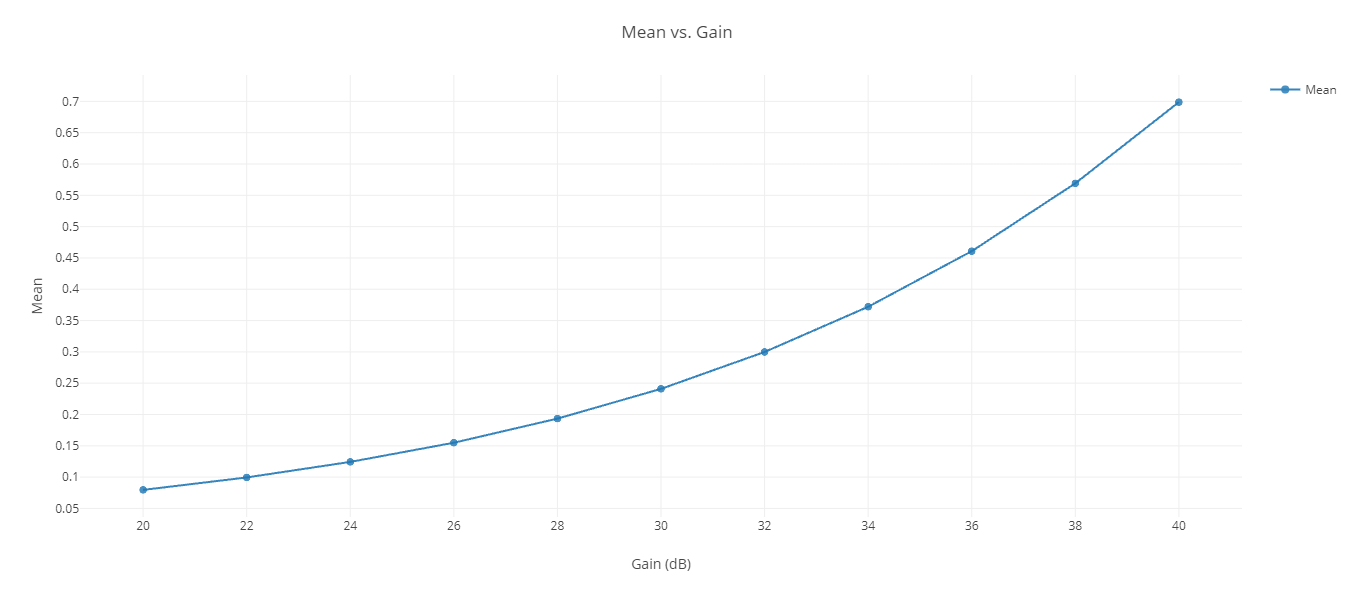
Mean S/T Integrated PDet vs. Gain 2D Line Plot
You can see from the study that the mean integrated probability of detection (S/T Integrated PDet) has a slight increase from a gain of 20 dB through 30 dB. However, from 30 dB through 40 dB, there is a steeper climb.
Closing out your trade study
Close out your trade study for the next section.
- Close the 2D Line Plot and the Table page when you are finished.
- Click when prompted to close your trade study without saving.
- Leave the Parametric Study tool open.
Studying goal signal-to-noise ratio (SNR)
Goal SNR is an integration analysis based on the desired signal-to-noise ratio. SNR is a measure that compares the level of a desired signal to the level of noise. The default value is 16 dB. Study how the SNR affects the mean value of integrated probability of detection.
Running a Parametric Study
Build a new Parametric Study using the SNR as your Design Variable.
- Click and drag SNR () from the Component Tree to the Design Variable field when the Parametric Study tool opens.
- Set the following Design Variable values:
- Click .
- Close the 2D Scatter Plot that automatically opened after the trade study finished running.
- Click Add View () on the Table Page toolbar.
- Select 2D Line Plot () in the drop-down menu.
This will replace Gain as the Design Variable.
| Option | Value |
|---|---|
| starting value | 10 |
| ending value | 22 |
| step size | 1 |
Setting options for the axes
Use the Axes tab to set options for the axes.
- Click Axes in the Plot Options menu.
- Select the Ticks tab.
- Change the Max # value to 20.
- Click anywhere on the plot to close the Plot Options menu.
- Review the 2D Line Plot.
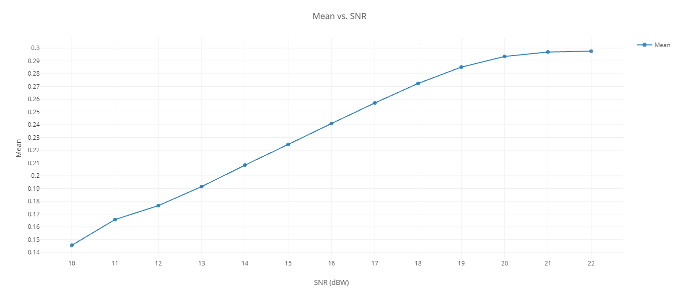
Mean S/T Integrated PDet vs. SNR 2D Line Plot
If you looking for a specific SNR, you can see the mean S/T Integrated PDet increases steadily until you reach approximately 20 dBW; at that level, it begins to taper off.
Closing out your trade study
Close out your trade study for the next section.
- Close the 2D Line Plot and the Table page when you are finished.
- Click when prompted to close your trade study without saving.
- Leave the Parametric Study tool open.
Studying the maximum pulses
Pulse integration is an improvement technique to address gains in probability of detection by using multiple transmit pulses. When a target is located within the radar beam during a single scan, it may reflect several pulses. By adding the returns from all pulses returned by a given target during a single scan, the radar sensitivity SNR can be increased. Most radars have a fixed number of pulses.
Running a Parametric Study
Build a new Parametric Study using the maximum pulses as your Design Variable.
- Click and drag MaximumPulses () from the Component Tree to the Design Variable field when the Parametric Study tool opens.
- Set the following Design Variable values:
- Click .
- Close the 2D Scatter Plot that automatically opened after the trade study finished running.
- Click Add View () on the Table Page toolbar.
- Select 2D Line Plot () in the drop-down menu.
- Review the 2D Line Plot.
This will replace SNR as the Design Variable.
| Option | Value |
|---|---|
| starting value | 1 |
| ending value | 200 |
| step size | 10 |
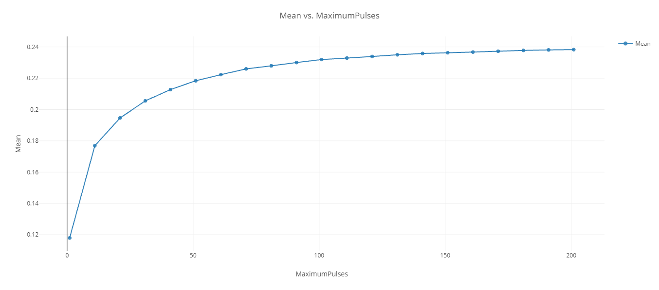
Mean S/T Integrated PDet vs. Maximum pulses Integrated 2D Line Plot
In this instance, the mean S/T Integrated PDet has a sharp rise until a maximum of 50 pulses integrated, after which it begins to level off.
Closing out your trade study
Close out your trade study for the next section.
- Close the 2D Line Plot and the Table page when you are finished.
- Click when prompted to close your trade study without saving.
- Close the Parametric Study tool.
Studying the gain and SNR together
You're looking for a combination of Gain and SNR that provide a mean S/T Integrated PDet value of 0.4 — that is, the average between 0.0 and 0.8. Find the value using a Carpet Plot.
Using the Carpet Plot tool
A Carpet Plot is a means of displaying data dependent on two variables in a format that makes interpretation easier than normal multiple curve plots. A Carpet Plot can be thought of as a multidimensional Parametric Study. Setting the design variables in a Carpet Plot is similar to using the Parametric Study tool except you now have two variables instead of one.
- Click Carpet Plot (
 ) on the Standard toolbar.
 - Click and drag Gain () from the Component Tree to the first Design Variables field when the Carpet Plot tool opens.
- Set the following Gain Design Variable values:
- Click and drag SNR () from the Component Tree to the second Design Variables field.
- Set the following SNR Design Variable values:
- Click and drag Mean () from the Component Tree to the Responses field.
- Click .
| Option | Value |
|---|---|
| From | 20 |
| To | 40 |
| Step Size | 5 |
| Option | Value |
|---|---|
| From | 10 |
| To | 20 |
| Step Size | 2 |
Setting options for the axes
Use the Axes tab to set options for the axes.
- Click Axes in the Plot Options menu.
- Select the Ticks tab.
- Change the Max # value to 40.
- Click anywhere on the plot to close the Plot Options menu.
Constraining the Carpet Plot
You can constrain the Carpet Plot for better visualization when looking for specific variable data.
- Click Constraints in the Plot Options menu.
- Set the following minimum values (the fields on the left) in the Constraints dialog box:
- When finished, click anywhere on the plot to close the Constraints menu.
- Review the Carpet Plot.
| Option | Value |
|---|---|
| Gain | 36 |
| SNR | 13.7 |
| Mean | 0.4 |
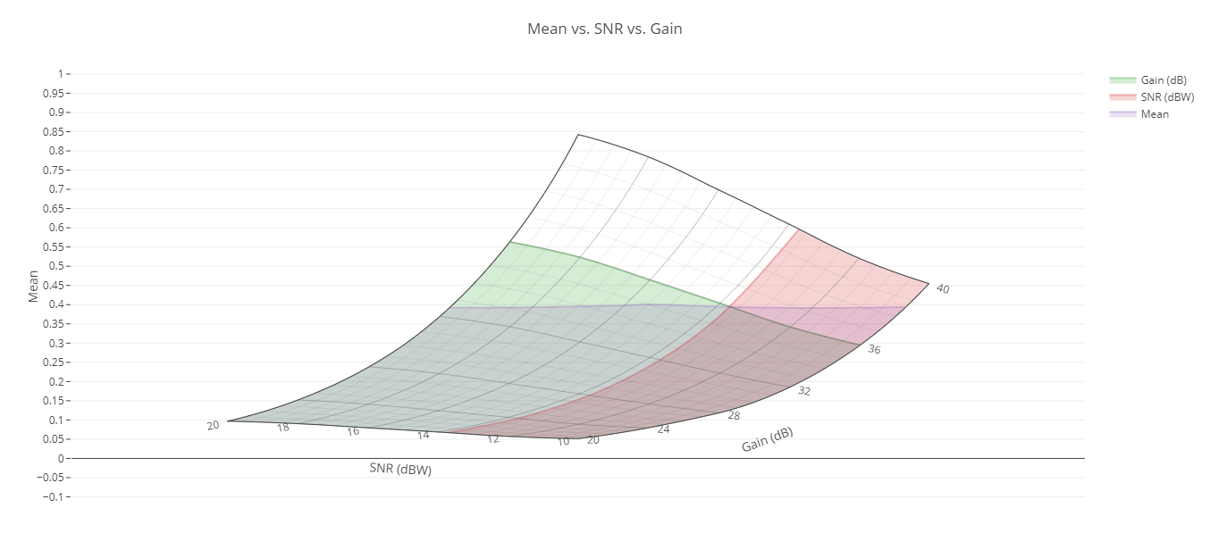
Mean S/T Integrated PDet vs SNR vs Gain Carpet Plot with constraints
You can see how the shading in the plot merge at an Integrated PDet of 0.4 when Gain is 36 dB and SNR is 13.7 dBW. You could have used the constraints dialog box and the slider bars to find the settings; the shading makes it easier to read the plot.
Saving your work
Save your work and close out ModelCenter application.
- Close out any open plots, tools, and the Data Explorer window.
- Click when prompted to close your trade study without saving.
- Click Save (
 ) to save your ModelCenter workflow.
 - Close the ModelCenter application.
Summary
You began by determining how long the multifunction radar could track an aircraft based on a S/T Integrated PDet value of 0.8 or higher. Using the ModelCenter software, you ran three different Parametric studies determining how gain, SNR and pulses integrated affect the mean value of S/T Integrated PDet. Finally, using the Carpet Plot tool, you determined which combination of gain and SNR provided a S/T Integrated PDet mean value of 0.4.
On your own
You can rerun all the Parametric studies using new values with the existing input variables. To make things interesting, you can study the MFR Multifunction inputs to see how they affect the mean S/T Integrated PDet. Likewise, if you look at the Access data provider variables, Radar Multifunction/TargetTransport has many more variables against which you can run additional trade studies.