STK Premium (Air), STK Premium (Space), or STK Enterprise
You can obtain the necessary licenses for this tutorial by contacting AGI Support at support@agi.com or 1-800-924-7244.
Required product install: The Ansys ModelCenter® model-based systems engineering software and the STK Plugin for ModelCenter are required to complete this tutorial.
ModelCenter installation prerequisites: The ModelCenter software requires the installation of a 64-bit version of Java, a 64-bit implementation of Python 3.x, and the installation of the thrift and six Python packages. See the ModelCenter Installation Prerequisites for more information.
This tutorial was written using version 2026 R1 of the Ansys ModelCenter® model-based systems engineering software.
The results of the tutorial may vary depending on the user settings and data enabled (online operations, terrain server, dynamic Earth data, etc.). It is acceptable to have different results.
Capabilities covered
This lesson covers the following capabilities of the Ansys Systems Tool Kit® (STK®) digital mission engineering software:
- STK Pro
- Coverage
- STK Analyzer
Problem statement
The Mount St. Helens Worm Flows Route, starting from the Marble Mountain Sno-Park (a cleared parking area for vehicles), is the most direct route to the summit of the Mount St. Helens during the winter season. It is also one of the most popular hiking and climbing routes up the volcano, which is located in the Cascades Range in the northwestern United States. Four ranger stations are used to visually observe the trail; occasionally, personnel limitations mean that only two stations can be crewed at a given time. You want to know which two observation posts, taken together, have the best percentage of visual coverage over the entire route.
Solution
Use the STK software's Coverage capability to analyze the coverage ability of the four ranger stations used to monitor the Mount St. Helens Worm Flows Route. Then, use the Analyzer capability, which is part of the Ansys ModelCenter® model-based systems engineering software, to perform a coverage analysis of the exercise area. You will perform a design of experiments (DOE) using all possible two-station combinations of the four different station locations to determine which two stations, taken together, provide the highest percentage of coverage along the hiking trail.
What you will learn
Upon completion of this tutorial, you will understand how to:
- Use a local analytical terrain file for analysis
- Import a KMZ file as a Line Target
- Use the Design of Experiments tool in the ModelCenter software
Creating a new scenario
First, you must create a new scenario, then build from there.
- Launch the STK (
 ) application.
 - Click
 Create a Scenario in the Welcome to STK dialog box.
 - Enter the following in the STK: New Scenario Wizard:
- Click when you finish.
- Click Save (
 ) when the scenario loads. STK creates a folder with the same name as your scenario for you.
 - Verify the scenario name and location in the Save As window.
- Click .
| Option | Value |
|---|---|
| Name | Ranger_Stations |
| Location | Default |
| Start | Default |
| Stop | Default |
Save (![]() ) often during this lesson!
) often during this lesson!
Configuring the terrain
You are performing analysis along the Mt. St. Helens Worm Flows Climbing Route. You would like to view the route and the surrounding terrain as a model in the 3D Graphics window. To do that, use the
Disabling streaming terrain
Since will import a local terrain file into your scenario, turn off Terrain Server for analysis.
- Right-click on Ranger_Stations () in the Object Browser.
- Select Properties (
 ).
). - Select the Basic - Terrain page.
- Clear the Use terrain server for analysis check box in the Terrain Server panel.
- Click to accept your changes and close the Properties Browser.
Importing a terrain file
Your STK software installation comes with a sample STK terrain (*.pdtt) file of the Mount St. Helens region. Use the
- Bring the 3D Graphics window to the front.
- Click Globe Manager (
 ) in the 3D Graphics window toolbar.
 - Click Add Terrain/Imagery (
 ) on the Globe Manager Hierarchy tab toolbar when the Globe Manager window opens.
 - Select the Add Terrain/Imagery... (
 ) option.
 - Click the Path ellipsis (
 ) when the Open Terrain and Imagery Data dialog box opens.
 - Navigate to <Install Dir>\Data\Resources\stktraining\imagery when the Browse For Folder dialog box opens.
- Click to confirm the directory selection and to close the Browse For Folder dialog box.
- Select the StHelens_Training.pdtt check box.
- Click .
- Click when prompted to use StHelens_Training.pdtt for analysis and to close the Open Terrain and Imagery Data dialog box.
Using a KMZ file in your scenario
You can use the
- Select the KML tab on the Globe Manager toolbar.
- Click Open KML Content (
 ) in the KML toolbar.
 - Go to <Install Dir>\Data\Resources\stktraining\KML.
- Select MtStHelens.kmz.
- Click .
Importing MtStHelens.kmz as an STK object
After you import the KMZ file into the STK application, you can import it as an object to use for your analysis. Since it is a path, import it as a
- Right-click on Mount St Helens Worm Flows Route (
 ) in the KML hierarchy.
 - Select Import as Line Target in the shortcut menu.
This will import the Mount St Helens Worm Flows Route as a Line Target object. Note that two placemarks are included in the KMZ file, represented as pushpins (![]() ) in the KML hierarchy. They mark the beginning and end of the route at Sno-Park (
) in the KML hierarchy. They mark the beginning and end of the route at Sno-Park ( ) in Marble Mountain and on the summit of Mount St. Helens in Gifford Pinchot National Forest (
 ), respectively.
Showing surface lines
Update your scenario's
- Open Ranger_Stations' () Properties ().
- Select the 3D Graphics - Global Attributes page.
- Open the On Terrain drop-down list in the Surface Lines panel.
- Select On.
- Click to accept your changes and to close the Properties Browser.
- Bring the 3D Graphics window to the front.
- Right-click on Mount_St_Helens_Worm_Flows_Route (
 ) in the Object Browser.
 - Select Zoom To in the shortcut menu.
- Move around in the 3D Graphics window to gain situational awareness about the route and terrain.
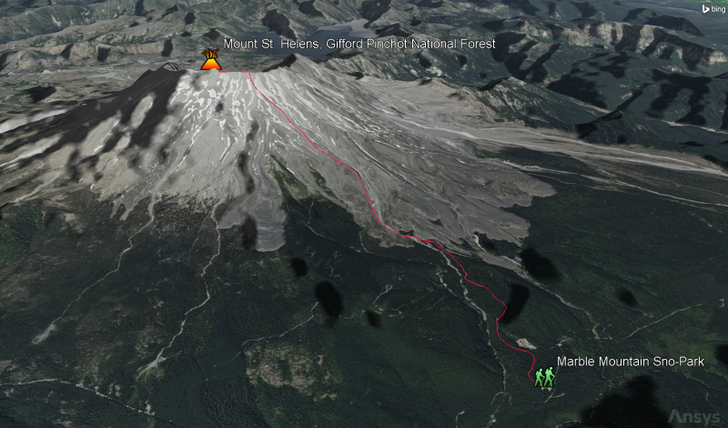
Mount st. Helens Worm Flows Route
Adding the ranger stations
There are four ranger stations along the hiking trail. These observation platforms are fifty feet high.
Building the first ranger station
You will build the first ranger station and then reuse it to create the other three ranger stations. By using Copy and Paste, all you will have to do is change the locations of the remaining three ranger stations.
- Bring the Insert STK Objects tool (
 ) to the front.
 - Insert a Place (
 ) object using the Define Properties () method.
 - Click .
- Set the following options on the Basic - Position page:
- Click to accept your changes and keep the Properties Browser open.
- Right-click on Place1 () in the Object Browser.
- Select Rename.
- Rename Place1 () Station1.
| Option | Value |
|---|---|
| Latitude | 46.1489 deg |
| Longitude | -122.177 deg |
| Height Above Ground | 50 ft |
Setting the constraints
Set viewing constraints on your ranger stations by using a
- Select the Constraints - Active page.
- Clear the Enable - Line Of Sight check box in the Active Constraints list.
- Click Add new constraints (
 ) in the Active Constraints toolbar.
 - Select Terrain Mask in the Constraint Name list when the Select Constraints to Add dialog box opens.
- Click .
- Click to close the Select Constraints to Add dialog box.
- Click to accept your changes and to close the Properties Browser.
Creating three more ranger stations
Using copy and paste, you can insert three more ranger stations into the scenario. You will only need to change their latitudes and longitudes.
- Select Station1 () in the Object Browser.
- Click Copy (
 ) in the Object Browser toolbar.
 - Click Paste (
 ) three times in the Object Browser toolbar.
 - One at a time, open the properties of Station2, Station3, and Station4, and make the following property changes on their Basic - Position page:
| Station | Latitude | Longitude |
|---|---|---|
| Station2 | 46.1412 deg | -122.165 deg |
| Station3 | 46.1638 deg | -122.184 deg |
| Station4 | 46.1606 deg | -122.174 deg |
Decluttering the labels
Use Label Declutter in the
- Bring the 3D Graphics window to the front.
- Click Properties () in the 3D Graphics window toolbar.
- Select the Details page in the Properties Browser.
- Select the Enable check box in the Label Declutter panel.
- Click to accept your changes and to close the Properties Browser.
Viewing the Worm Flows route and the ranger stations
Use the 3D Graphics window to view the route and ranger stations in context to gain better situational awareness.
- Bring the 3D Graphics window to the front.
- Right click on Station1 () in the Objects Browser
- Select Zoom To in the shortcut menu.
- Move around in the 3D Graphics window and zoom out until you can see the Worm Flows Route and all four ranger stations.
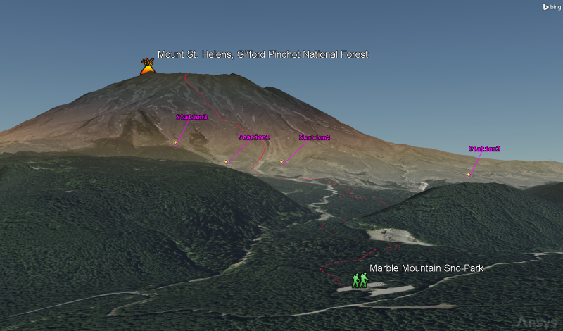
Ranger stations Along Worm Flows Route
Assessing coverage
The STK software's
Defining the Grid Area of Interest
You want to assess the coverage of any two of the four nodes (that is, the ranger stations) along Mount St. Helens Worm Flows route. Coverage analyses are based on the accessibility of assets (objects that provide coverage) and geographical areas. For analysis purposes, you can refine the geographical areas of interest using regions and points. Points have specific geographical locations, and the STK software uses them in the computation of asset availability. Regions are closed boundaries that contain points. The STK software computes accessibility to a region based on accessibility to the points within that region. The combination of the geographical area, the regions within that area, and the points within each region is called the
Use a
- Bring the Insert STK Objects tool () to the front.
- Insert a Coverage Definition (
 ) object using the Insert Default () method.
 - Open CoverageDefinition1's (
 ) Properties ().
 - Ensure the Basic - Grid page is selected.
- Select Custom Boundary in the Type drop-down list in the Grid Area of Interest panel.
- Click.
- Select Mount_St_Helens_Worm_Flows_Route () in the Boundary Objects list when the Select Boundaries... dialog box opens.
- Move (
 ) Mount_St_Helens_Worm_Flows_Route () from the Boundary Objects list to the Selected Objects list.
 - Click to confirm your selection and to close the Select Boundaries... dialog box.
Specifying the point granularity
The statistical data computed during a coverage analysis is based on a set of locations, or points, that span the specified grid area of interest. Set the exact location of the grid points based on a specified granularity by updating the grid's point granularity options.
- Select Distance in the Point Granularity shortcut menu in the Grid Definition panel.
- Enter 10 ft in the Distance field.
The Distance option defines the location of the grid coordinates by using the specified distance to determine a latitude / longitude spacing scheme at the equator.
Specifying the point altitude
Place the grid points to 5 feet above the terrain.
- Select Altitude above Terrain in the Point Altitude drop-down list.
- Enter 5 ft in the Altitude above Terrain field.
- Click to accept your changes and to keep the Properties Browser open.
The height will be a constant five-foot offset from the terrain, which varies with the latitude and longitude of each grid point.
Setting your grid constraints
Once you have defined the grid area, you can specify an object class or a specific object for the points within the grid. If you select an object, the constraints set for the object are also used by all the points within the grid. Use the constraints you applied to Station1 to apply
- Click in the Grid Definition panel.
- Select Place in the Reference Constraint Class drop-down list in the Grid Point Access Options panel when the Grid Constraint Options dialog box opens.
- Select the Use Object Instance check box.
- Select Station1.
- Click to confirm your selection and to close the Grid Constraint Options dialog box.
- Click to accept your changes and keep the Properties Browser open.
Selecting your coverage assets
Assets properties enable you to specify the STK objects you want to use to provide coverage.
- Select the Basic - Assets page in the Coverage Properties Browser.
- Multi-select all four Place () objects in the Assets list.
- Click .
- Note the status of each asset is Active.
- Click to accept your changes and keep the Properties Browser open.
You can set a coverage asset's status either to Active or to Inactive. This enables you to remove selected assets from consideration without removing access information from the coverage calculations, and is typically useful after accesses have been computed. You will use this status to perform a trade study in ModelCenter.
Defining the coverage interval
For your scenario, you have static assets covering a static area. If you compute the coverage over the whole scenario time, that would be a waste of computational time. None of the objects will change positions over time, so you can significantly shorten the computation time. Specify the
- Select the Basic - Interval page.
- Open the Interval drop-down menu (
 ) in the Access Interval panel.
 - Select Replace With Times.
- Leave the Start of the interval the default time.
- Enter +1 sec in the Stop field.
- Click to accept your changes and keep the Properties Browser open.
Disabling automatically recompute accesses
Advanced properties enable you to adjust the manner in which STK stores and computes access information. Although it is not required, the possibility exists that after computing coverage, you might change the properties of an asset. Therefore, set up the Coverage Definition object to enable you to manually compute coverage by updating your coverage definition's
- Select the Basic - Advanced page.
- Clear the Automatically Recompute Accesses check box in the Access panel.
- Click to accept your changes and keep the Properties Browser open.
Showing the 2D Graphics coverage grid
Later in the scenario, you will display color contours along the route. In order to better visualize the contour colors, you can remove the grid points along the route.
- Select the 2D Graphics - Attributes page.
- Clear the Show Points check box in the Grid panel.
- Click to accept your changes and close the Properties Browser.
Computing accesses
The ultimate goal of coverage is to analyze accesses to an area using assigned assets and applying necessary limitations upon those accesses. Several tools are available to the Coverage Definition object that will assist you in computing, reloading, clearing, and exporting access calculations. Accesses can only be computed for a coverage definition; the
- Select CoverageDefinition1 () in the Object Browser.
- Select CoverageDefinition in the Menu Bar.
- Select Compute Accesses in the CoverageDefinition menu.
Evaluating the quality of coverage with a figure of merit
You can evaluate the quality of coverage for an area by creating a Figure Of Merit object attached to the coverage definition of interest.
Creating a new Figure of Merit
A
- Insert a Figure of Merit (
 ) object using the Insert Default () method.
 - Select CoverageDefinition1 () in the Select Object dialog box.
- Click to confirm your selection and to close the Select Object dialog box.
Measuring the number of assets
Prior to running a trade study with the ModelCenter software, you need to determine how much of the route can be observed when all four stations are manned. Use an
- Open FigureOfMerit1's () Properties ().
- Select the Basic - Definition page.
- Select N Asset Coverage in the Definition - Type drop-down list.
- Set the following satisfaction criterion options in the Satisfaction panel:
- Click to accept your changes and keep the Properties Browser open.
| Option | Action |
|---|---|
| Enable | Selected |
| Satisfied if | Greater Than |
| Threshold | 0 |
Changing the criterion and threshold will determine which accesses are considered valid.
Turning off animation graphics
In the Figure of Merit properties, the
- Return to the Figure of Merit () object's Properties ().
- Select the 2D Graphics - Animation page.
- Clear the Show Animation Graphics check box.
- Click to accept your changes and keep the Properties Browser open.
Generating a Percent Satisfied report
You want to determine the overall percentage of coverage along the route when all of the ranger stations are manned. A
- Right-click on FigureOfMerit1 () in the Object Browser.
- Select Report & Graph Manager... (
 ) in the shortcut menu.
 - Select the Percent Satisfied (
 ) report in the Styles (
 ) folder in the Report & Graph Manager.
 - Click .
- Note the % Satisfied statistic at the bottom of the report.
- Close the report and the Report & Graph Manager.
The route is approximately 93 percent satisfied when all four stations are utilized. You'll compare this number to your analysis by using the ModelCenter application.
Creating static contours
You can specify how levels of coverage quality display in both the 2D and 3D Graphics windows. To accurately display contour levels for figures of merit in the 2D and 3D Graphics window, you should know the approximate range of values for the current Figure Of Merit. You have four stations in your coverage analysis. Based on your Percentage Satisfied report, you don't have 100% coverage. There are obvious gaps in the coverage, so you need to create a contour range.
- Select the 2D Graphics - Static page.
- Select the Markers check box in the Show Points As panel.
- Leave the default marker as is.
- Select the Show Contours check box in the Display Metric panel.
- Click in the Level Attributes panel.
- Set the following options in the Level Adding panel:
- Click .
- Ensure Color Ramp is selected in the Color Method shortcut menu.
- Set the following level attribute options:
- Click to accept your changes and to keep the Properties Browser open.
The
| Option | Value |
|---|---|
| Start | 0 |
| Stop | 4 |
| Step | 1 |
| Option | Value |
|---|---|
| Start Color | Red |
| End Color | Blue |
Displaying a contour legend in the 2D Graphics window
A contour key, or legend, provides you with a convenient way to interpret contour data displayed in the 2D and 3D Graphics windows. In this instance, you cannot view the Line Target object contours in the 2D Graphics window.
- Click .
- Click in the Static Legend for FigureOfMerit1 dialog box.
- Select the Show at Pixel Location check box in the 2D Graphics Window panel when the Figure of Merit Legend Layout dialog box opens.
- Enter 0 in the Number Of Decimal Digits field in the Text Options panel.
- Click to close the Figure of Merit Legend Layout dialog box.
- Close the Static Legend for FigureOfMerit1 dialog box.
- Click to accept your changes and to close the Properties Browser.
- Bring the 2D Graphics window to the front. You should see the legend in the window.
- Using your mouse, zoom in to the Worm Flows Route.
The
You should see the color contours representing how many stations can simultaneously observe that portion of the route.
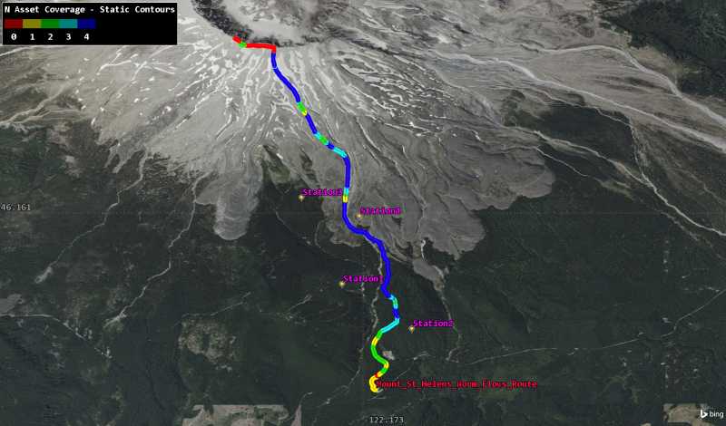
Coverage Color Contours
Creating a new ModelCenter project
The
- Save () your scenario.
- Close any open reports, the Report & Graph Manager, and any open tools.
- Close the STK application.
- Open the ModelCenter (
 ) application.
 - Click in the Welcome to ModelCenter dialog box.
- Click when the What type of model would you like to create? dialog box opens.
- Navigate to your scenario folder (for example, C:\Users\<username>\Documents\STK_ODTK 13\Ranger_Stations.
- Enter Ranger_Stations in the File name field.
- Ensure the Save as type is set to the ModelCenter Model (Zip) (*.pxcz).
- Click .
Configuring the STK Plugin for ModelCenter
The
- Select favorites (
 ) in the Server Browser at the bottom of the window.
 - Click and drag the STK component (
 ) into the dashed circle underneath "Drop items here to build the model" in the workflow's Analysis View.
 - Select Ranger_Stations.sc when the Open STK Scenario file dialog box opens.
- Click .
- After a few moments, the STK Analyzer window will open.
The Ranger_Stations scenario file will open in the STK application in the background.
You can add any of the STK variables as ModelCenter input or output variables through the STK Analyzer window that appears. If you change the value of a variable in your scenario through the STK interface or the ModelCenter Component Tree, you should re-add the variable into ModelCenter or re-run the workflow before running any trade studies with the new value.
Evaluating coverage ability using Analyzer
Now that you have determined the static coverage values for the route, use the Design of Experiments tool to perform a trade study to determine which two nodes will result in the least degradation.
Selecting the input variables
Use the STK Analyzer window to configure the input and output variables available for further analysis with the
- Select CoverageDefinition1 () in the STK Variables tree.
- Expand (
 ) the Assets (
 ) property.
 - Expand () the Place/Station1 () property.
- Select Status (
 ).
). - Move (
 ) Status () to the Analyzer Variables list.
 - Repeat the process for Place/Station2 () through Place/Staiton4, moving all four Status () to the Analyzer Variables list.
When you select an object in the STK Variables tree, all possible input variable candidates for that object are listed under the General tab and the Active Constraints tab in the STK Property Variables panel.
Selecting the output variable
The same data providers that are available in the Report & Graph Manager in the STK application are available in the Data Provider Variables tree.
- Select FigureOfMerit1 () in the STK Variables tree.
- Expand () the Static Satisfaction (
 ) data provider.
 - Select the Percent Satisfied (
 ) data provider element.
 - Move () Percent Satisfied () to the Analyzer Variables list.
- Click to confirm your selections and to close the STK Analyzer window.
Note that Percent Satisfied ( ) is listed under Outputs in the Analyzer Variables list. You now have the required inputs and outputs for the trade study.
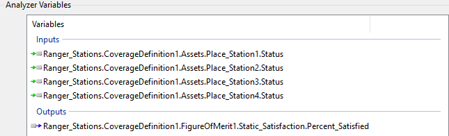
Analyzer Variables
This will also close the STK application, which had been running in the background.
Using the Design of Experiments tool
The DOE (Design of Experiments) Tool simplifies the purposeful changing of inputs (design variables) in a model to observe the corresponding changes in outputs (response variables). A set of valid values for each design variable constitutes a design point. Use this tool to collect the responses in the model to a set of predetermined design points. Tools are provided to graphically set up and conduct this experiment.
For this exercise, you need to cover all possibilities of two stations being manned and two stations being unmanned. You are determining which pair of stations will provide the highest percentage of coverage.
- Expand (
 ) all the elements in the Component Tree.
 - Click DOETool (
 ) on the Standard toolbar.
 - Click and drag Place_Station1's Status (
 ) variable to the Design Variables field when the DOE Tool opens.
 - Repeat the step above for the Place_Station2, Place_Station3, and Place_Station4 Status () variables.
- Note that the variable values are listed as being Enumerated, with two possible values: eActive and eInactive.
- Drag and drop Percent_Satisfied (
 ) from the Components list to the Responses list.
 - Click to perform the study.
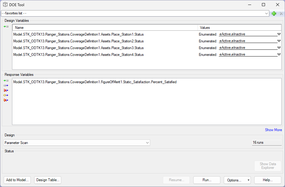
DOE Tool setup
When the DOE study is run, it will repeatedly set the value for the design variables and then validate each of the response variables It will open the Data Explorer, which is a tool used by Trade Study tools to display data collected from a Model. While data are being collected, the Data Explorer displays a progress meter, a halt button, and the data.
Reviewing the results in the Data Explorer
The Table page of the Data Explorer displays trade study data in a tabular form. It is the default window that is present for all trade studies. Cells are shaded differently depending on the associated variable's state. Input variables are shown with green text, valid values are displayed with black text, invalid values are displayed with gray text, and modified values are displayed with blue text. From the table it is possible to view and edit all values in your trade study and even to add and remove whole runs. You can use the Chart menu options to help you identify which has the highest percentage of coverage for two active ranger stations.
- Select the response(Model.STK_ODTK13.Ranger_Stations.CoverageDefinition1.FigureOfMerit1.Static_Statisfaction.Percent_Satisfied) row in the Data Explorer table.
- Select the Chart menu.
- Select Sort Descending.
- Review the results.
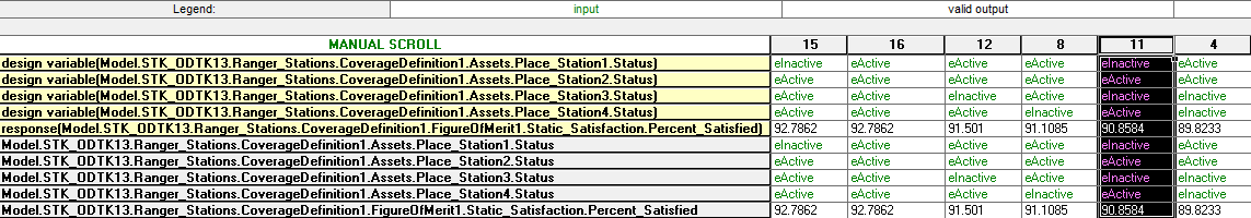
Table of runs with best two-station run selected
You can see that, as expected, the runs with the highest percentage of coverage are those with three and four stations manned (that is, with a status of eActive) with a coverage of approximately 93% of the trail. However, when only Station2 and Station4 are crewed, they together can cover approximately 91% of the trail. Therefore, on days that only allow two ranger stations to operate, using stations two and four are the best choice for a minimal degradation in your coverage ability.
Saving your work
Save your work and close out ModelCenter application.
- Close out any open plots, tools, and the Data Explorer window.
- Click when prompted to close your trade study without saving.
- Click Save (
 ) to save your ModelCenter workflow.
 - Close the ModelCenter application.
De-assigning stations one and three
Using the run that resulted in the highest percentage of coverage along the route, you can change the Coverage Definition object's assigned assets to reflect and visualize the coverage along the route.
- Reopen the STK application ().
- Reopen your Ranger_Stations scenario file.
- Open CoverageDefinition1's () Properties ().
- Select the Basic - Assets page when the Properties Browser opens.
- Multi-select Station1 () and Station3 () in the Assets list.
- Select Inactive in the Status list.
- Click to accept your changes and to close the Properties Browser.
- Bring the 2D Graphics window to the front to view the overall coverage using just Station2 () and Station4 ().
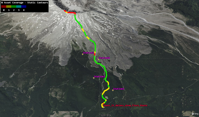
Station 2 and station 4 coverage Contours
You can see that the majority of the route is covered by at least one ranger station, with the areas that are unable to be seen from either station occurring in deep valleys or over the rim of the volcano.
Saving your work
Save your work and close out of the STK application.
- Close any open reports, properties, and the Report & Graph Manager.
- Save () your work.
- Close the STK application.
Summary
This tutorial introduced you to the Design of Experiments tool in ModelCenter and how you can use it to aid in assigning coverage assets. By importing a local analytical file as a terrain inlay and converting a KMZ file into a Line Target object, you were able to model your coverage area of interest with high fidelity. You utilized the STK software's Coverage capability to obtain the percentage of route, which was visible from four assigned coverage assets. Using the ModelCenter software's Design of Experiments tool, you determined that comparable coverage could be obtained with just two of the four assets being used. By using the ModelCenter software, you can quickly and easily economize your design space and test assets.